Seurat’s AddModuleScore function

Last updated: 2025-02-19

Checks: 7 0

Knit directory: muse/

This reproducible R Markdown analysis was created with workflowr (version 1.7.1). The Checks tab describes the reproducibility checks that were applied when the results were created. The Past versions tab lists the development history.

R Markdown file: up-to-date

Great! Since the R Markdown file has been committed to the Git repository, you know the exact version of the code that produced these results.

Environment: empty

Great job! The global environment was empty. Objects defined in the global environment can affect the analysis in your R Markdown file in unknown ways. For reproduciblity it’s best to always run the code in an empty environment.

Seed: set.seed(20200712)

The command set.seed(20200712) was run prior to running the code in the R Markdown file. Setting a seed ensures that any results that rely on randomness, e.g. subsampling or permutations, are reproducible.

Session information: recorded

Great job! Recording the operating system, R version, and package versions is critical for reproducibility.

Cache: none

Nice! There were no cached chunks for this analysis, so you can be confident that you successfully produced the results during this run.

File paths: relative

Great job! Using relative paths to the files within your workflowr project makes it easier to run your code on other machines.

Repository version: a18365d

Great! You are using Git for version control. Tracking code development and connecting the code version to the results is critical for reproducibility.

The results in this page were generated with repository version a18365d. See the Past versions tab to see a history of the changes made to the R Markdown and HTML files.

Note that you need to be careful to ensure that all relevant files for the analysis have been committed to Git prior to generating the results (you can use wflow_publish or wflow_git_commit). workflowr only checks the R Markdown file, but you know if there are other scripts or data files that it depends on. Below is the status of the Git repository when the results were generated:


Ignored files:
    Ignored:    .Rproj.user/
    Ignored:    data/1M_neurons_filtered_gene_bc_matrices_h5.h5
    Ignored:    data/293t/
    Ignored:    data/293t_3t3_filtered_gene_bc_matrices.tar.gz
    Ignored:    data/293t_filtered_gene_bc_matrices.tar.gz
    Ignored:    data/5k_Human_Donor1_PBMC_3p_gem-x_5k_Human_Donor1_PBMC_3p_gem-x_count_sample_filtered_feature_bc_matrix.h5
    Ignored:    data/5k_Human_Donor2_PBMC_3p_gem-x_5k_Human_Donor2_PBMC_3p_gem-x_count_sample_filtered_feature_bc_matrix.h5
    Ignored:    data/5k_Human_Donor3_PBMC_3p_gem-x_5k_Human_Donor3_PBMC_3p_gem-x_count_sample_filtered_feature_bc_matrix.h5
    Ignored:    data/5k_Human_Donor4_PBMC_3p_gem-x_5k_Human_Donor4_PBMC_3p_gem-x_count_sample_filtered_feature_bc_matrix.h5
    Ignored:    data/Parent_SC3v3_Human_Glioblastoma_filtered_feature_bc_matrix.tar.gz
    Ignored:    data/brain_counts/
    Ignored:    data/cl.obo
    Ignored:    data/cl.owl
    Ignored:    data/jurkat/
    Ignored:    data/jurkat:293t_50:50_filtered_gene_bc_matrices.tar.gz
    Ignored:    data/jurkat_293t/
    Ignored:    data/jurkat_filtered_gene_bc_matrices.tar.gz
    Ignored:    data/pbmc3k/
    Ignored:    data/pbmc4k_filtered_gene_bc_matrices.tar.gz
    Ignored:    data/refdata-gex-GRCh38-2020-A.tar.gz
    Ignored:    data/seurat_1m_neuron.rds
    Ignored:    data/t_3k_filtered_gene_bc_matrices.tar.gz
    Ignored:    r_packages_4.4.1/

Note that any generated files, e.g. HTML, png, CSS, etc., are not included in this status report because it is ok for generated content to have uncommitted changes.

These are the previous versions of the repository in which changes were made to the R Markdown (analysis/add_module_score.Rmd) and HTML (docs/add_module_score.html) files. If you’ve configured a remote Git repository (see ?wflow_git_remote), click on the hyperlinks in the table below to view the files as they were in that past version.

File	Version	Author	Date	Message
Rmd	a18365d	Dave Tang	2025-02-19	Remove clusters and check module scores
html	15d797c	Dave Tang	2025-02-19	Build site.
Rmd	640394d	Dave Tang	2025-02-19	Include a summary
html	99e85e1	Dave Tang	2025-02-19	Build site.
Rmd	55128f2	Dave Tang	2025-02-19	Seurat’s add module score

A bastardisation of Walter Muskovic’s blog post Seurat’s AddModuleScore function (my apologies).

Load packages.

suppressPackageStartupMessages(library("Seurat"))
suppressPackageStartupMessages(library("ggplot2"))

Download the Peripheral Blood Mononuclear Cells (PBMCs) 2,700 cells dataset.

mkdir -p data/pbmc3k && cd data/pbmc3k
wget -c https://s3-us-west-2.amazonaws.com/10x.files/samples/cell/pbmc3k/pbmc3k_filtered_gene_bc_matrices.tar.gz
tar -xzf pbmc3k_filtered_gene_bc_matrices.tar.gz

Create Seurat object.

work_dir <- rprojroot::find_rstudio_root_file()
data_dir <- paste0(work_dir, "/data/pbmc3k/filtered_gene_bc_matrices/hg19/")
stopifnot(dir.exists(data_dir))
pbmc.data <- Read10X(
  data.dir = data_dir
)

seurat_obj <- CreateSeuratObject(
  counts = pbmc.data,
  min.cells = 3,
  min.features = 200,
  project = "pbmc3k"
)

Warning: Feature names cannot have underscores ('_'), replacing with dashes
('-')

debug_flag <- FALSE
seurat_obj <- NormalizeData(seurat_obj, normalization.method = "LogNormalize", scale.factor = 1e4, verbose = debug_flag)
seurat_obj <- FindVariableFeatures(seurat_obj, selection.method = 'vst', nfeatures = 2000, verbose = debug_flag)
seurat_obj <- ScaleData(seurat_obj, verbose = debug_flag)
seurat_obj <- RunPCA(seurat_obj, verbose = debug_flag)
seurat_obj <- RunUMAP(seurat_obj, dims = 1:30, verbose = debug_flag)

Warning: The default method for RunUMAP has changed from calling Python UMAP via reticulate to the R-native UWOT using the cosine metric
To use Python UMAP via reticulate, set umap.method to 'umap-learn' and metric to 'correlation'
This message will be shown once per session

seurat_obj <- FindNeighbors(seurat_obj, dims = 1:30, verbose = debug_flag)
seurat_obj <- FindClusters(seurat_obj, resolution = 0.5, verbose = debug_flag)

seurat_obj

An object of class Seurat 
13714 features across 2700 samples within 1 assay 
Active assay: RNA (13714 features, 2000 variable features)
 3 layers present: counts, data, scale.data
 2 dimensional reductions calculated: pca, umap

UMAP.

DimPlot(seurat_obj, label = TRUE, repel = TRUE) + NoLegend()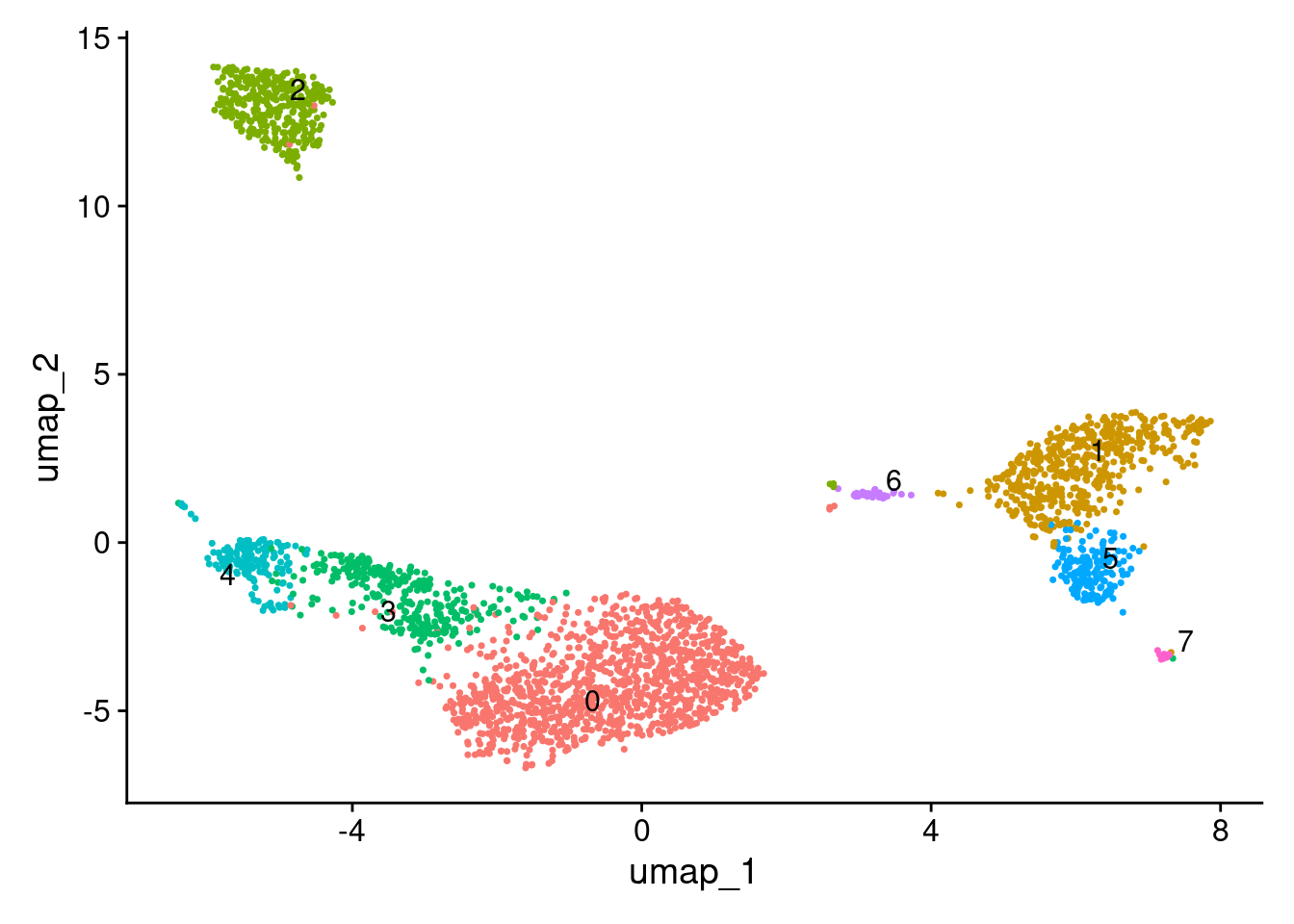

Version	Author	Date
99e85e1	Dave Tang	2025-02-19

Get top 20 genes enriched in cluster 4.

FindMarkers(seurat_obj, ident.1 = "4", verbose = FALSE) |>
  tibble::rownames_to_column(var = "gene_symbol") |>
  head(20) |>
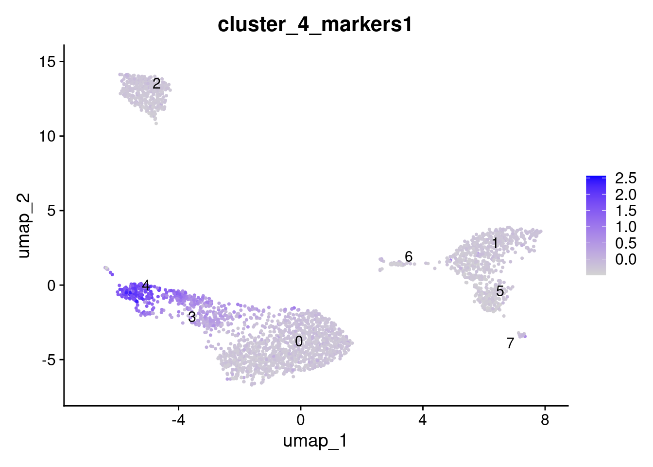
  dplyr::pull(gene_symbol) -> cluster_4_markers

Add module score; it is very important that features are provided as a list.

AddModuleScore(
  seurat_obj,
  features = list(cluster_4_markers),
  name = "cluster_4_markers"
) -> seurat_obj

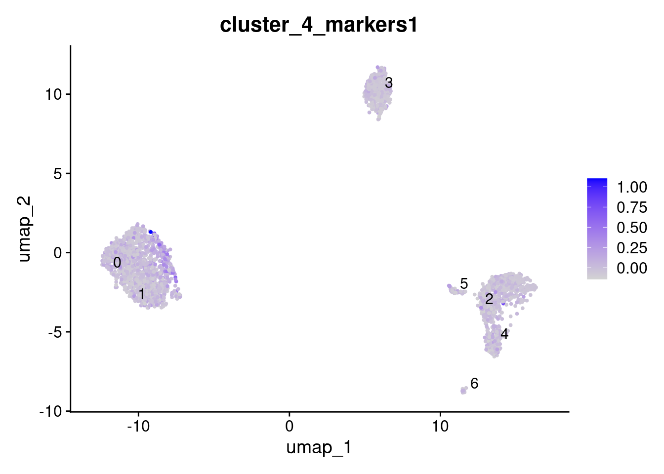
FeaturePlot(
  seurat_obj,
  features = "cluster_4_markers1",
  label = TRUE,
  repel = TRUE
)

Version	Author	Date
99e85e1	Dave Tang	2025-02-19

Details of method in the supplementary materials:

The top 100 MITF-correlated genes across the entire set of malignant cells were defined as the MITF program, and their average relative expression as the MITF-program cell score.
The average expression of the top 100 genes that negatively correlate with the MITF program scores were defined as the AXL program and used to define AXL program cell score.
To decrease the effect that the quality and complexity of each cell’s data might have on its MITF/AXL scores we defined control gene-sets and their average relative expression as control scores, for both the MITF and AXL programs.
These control cell scores were subtracted from the respective MITF/AXL cell scores.
The control gene-sets were defined by first binning all analyzed genes into 25 bins of aggregate expression levels and then, for each gene in the MITF/AXL gene-set, randomly selecting 100 genes from the same expression bin as that gene.
In this way, a control gene-sets have a comparable distribution of expression levels to that of the MITF/AXL gene-set and the control gene set is 100-fold larger, such that its average expression is analogous to averaging over 100 randomly-selected gene-sets of the same size as the MITF/AXL gene-set.

Implementation in Seurat.

object <- seurat_obj
features <- list(cluster_4_markers)
pool <- rownames(seurat_obj)
nbin <- 24
ctrl <- 100
k <- FALSE
name = "cluster_4_markers"
seed = 1

# Find how many gene lists were provided. In this case just one.
cluster.length <- length(x = features)
cluster.length

[1] 1

# Pull the expression data from the provided Seurat object
# uses DefaultAssay()
# default is the data layer, by order
assay.data <- GetAssayData(object = object)
class(assay.data)

[1] "dgCMatrix"
attr(,"package")
[1] "Matrix"

# For all genes, get the average expression across all cells (named vector)
data.avg <- Matrix::rowMeans(x = assay.data[pool, ])
length(data.avg)

[1] 13714

# Order genes from lowest average expression to highest average expression
data.avg <- data.avg[order(data.avg)]
head(data.avg)

        CDC6       SHCBP1       VPREB1        ESCO2         LHFP          PBK 
0.0007395302 0.0010637455 0.0010654207 0.0010927958 0.0011109484 0.0011122871

# Use ggplot2's cut_number function to make n groups with (approximately) equal numbers of observations.
# The 'rnorm(n = length(data.avg))/1e+30' part adds a tiny bit of noise to the data, presumably to break ties.
# similar to base R's cut function
data.cut <- ggplot2::cut_number(
  x = data.avg + rnorm(n = length(data.avg))/1e+30,
  n = nbin,
  labels = FALSE,
  right = FALSE
)
table(data.cut)

data.cut
  1   2   3   4   5   6   7   8   9  10  11  12  13  14  15  16  17  18  19  20 
572 571 572 571 571 572 571 571 572 571 572 571 571 572 571 571 572 571 572 571 
 21  22  23  24 
571 572 571 572

# Set the names of the cuts as the gene names
names(x = data.cut) <- names(x = data.avg)
head(data.cut)

  CDC6 SHCBP1 VPREB1  ESCO2   LHFP    PBK 
     1      1      1      1      1      1

# Create an empty list the same length as the number of input gene sets.
# This will contain the names of the control genes
ctrl.use <- vector(mode = "list", length = cluster.length)

# For each of the input gene lists:
for (i in 1:cluster.length) {
  # Get the gene names from the input gene set as a character vector  
  features.use <- features[[i]]
  
  # Loop through the provided genes (1:num_genes)
  # for each gene, find ctrl (default=100) genes from the same expression bin (by looking in data.cut):
  for (j in 1:length(x = features.use)) {
    # Within this loop, 'data.cut[features.use[j]]' gives us the expression bin number.
    # We then sample `ctrl` genes from that bin without replacement and add the gene names to ctrl.use.
    ctrl.use[[i]] <- c(
      ctrl.use[[i]],
      names(x = sample(
        x = data.cut[which(x = data.cut == data.cut[features.use[j]])],
        size = ctrl,
        replace = FALSE)
      )
    )
  }
}

# Have a quick look at what's in ctrl.use:
class(ctrl.use)

[1] "list"

length(ctrl.use)

[1] 1

class(ctrl.use[[1]])

[1] "character"

# There should be length(features.use)*ctrl genes (i.e. 20*100):
length(ctrl.use[[1]])

[1] 2000

head(ctrl.use[[1]])

[1] "NOL7"     "SDHC"     "TNFRSF14" "RNPS1"    "SUPT4H1"  "CHMP2A"

Explanatory plot.

# Plot the bins that have been created to split genes based on their average expression
plot(data.avg, pch=16, ylab="Average expression across all cells", xlab="All genes, ranked")

for(i in unique(data.cut)){
  cut_pos <- which(data.cut==i)
  if(i%%2==0){
    rect(xleft = cut_pos[1], ybottom = min(data.avg), xright = cut_pos[length(cut_pos)], ytop = max(data.avg), col=scales::alpha("grey", 0.3))
  } else {
    rect(xleft = cut_pos[1], ybottom = min(data.avg), xright = cut_pos[length(cut_pos)], ytop = max(data.avg), col=scales::alpha("white", 0.3))
  }
}

# Add red points for selected control genes
points(which(names(data.avg)%in%ctrl.use[[1]]), data.avg[which(names(data.avg)%in%ctrl.use[[1]])], pch=16, col="red")

# Add blue points for genes in the input gene list
points(which(names(data.avg)%in%features[[1]]), data.avg[which(names(data.avg)%in%features[[1]])], pch=16, col="blue")

# Add a legend
legend(x = "topleft",
       legend = c("gene", "selected control gene", "gene in geneset"),
       col = c("black", "red", "blue"),
       pch = 16)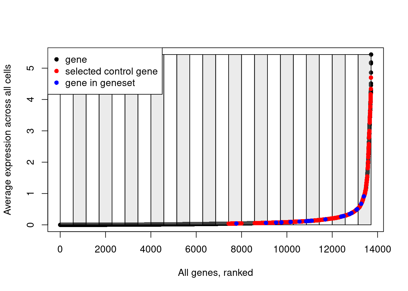

Version	Author	Date
99e85e1	Dave Tang	2025-02-19

Note how control genes are only selected from the bins in which the genes in our input list fall.

# Remove any repeated gene names - even though we set replace=FALSE when we sampled genes from the same expression bin, there may be more than two genes in our input gene list that fall in the same expression bin, so we can end up sampling the same gene more than once.
ctrl.use <- lapply(X = ctrl.use, FUN = unique)

## Get control gene scores

# Create an empty matrix with dimensions:
#     number of rows equal to the number of gene sets (just one here)
#     number of columns equal to number of cells in input Seurat object
ctrl.scores <- matrix(
  data = numeric(length = 1L),
  nrow = length(x = ctrl.use),
  ncol = ncol(x = object)
)
dim(ctrl.scores)

[1]    1 2700

# Loop through each provided gene set and add to the empty matrix the mean expression of the control genes in each cell
for (i in 1:length(ctrl.use)) {
  # Get control gene names as a vector  
  features.use <- ctrl.use[[i]]
  # For each cell, calculate the mean expression of *all* of the control genes 
  ctrl.scores[i, ] <- Matrix::colMeans(x = assay.data[features.use,])
}

## Get scores for input gene sets

# Similar to the above, create an empty matrix
features.scores <- matrix(
  data = numeric(length = 1L),
  nrow = cluster.length,
  ncol = ncol(x = object)
)
dim(features.scores)

[1]    1 2700

# Loop through input gene sets and calculate the mean expression of these genes for each cell
for (i in 1:cluster.length) {
  features.use <- features[[i]]
  data.use <- assay.data[features.use, , drop = FALSE]
  features.scores[i, ] <- Matrix::colMeans(x = data.use)
}

Now we have two matrices:

ctrl.scores - contains the mean expression of the control genes for each cell
features.scores - contains the mean expression of the genes in the input gene set for each cell

Now to calculate the scores.

# Subtract the control scores from the feature scores
# the idea is that if there is no enrichment of the genes in the geneset in a cell, then the result of this subtraction should be ~ 0
features.scores.use <- features.scores - ctrl.scores

# Name the result the "name" variable + whatever the position the geneset was in the input list, e.g. "Cluster1"
rownames(x = features.scores.use) <- paste0(name, 1:cluster.length)

# Change the matrix from wide to long
features.scores.use <- as.data.frame(x = t(x = features.scores.use))

# Give the rows of the matrix, the names of the cells
rownames(x = features.scores.use) <- colnames(x = object)

# Add the result as a metadata column to the input Seurat object 
object[[colnames(x = features.scores.use)]] <- features.scores.use

# Voila!
FeaturePlot(object, features = "cluster_4_markers1", label = TRUE)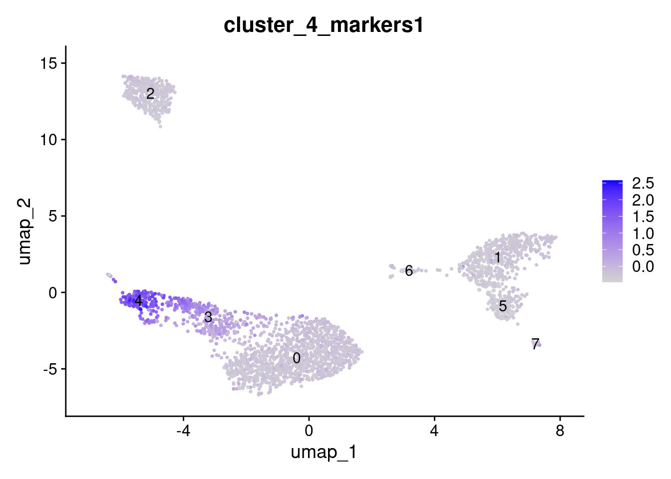

Version	Author	Date
15d797c	Dave Tang	2025-02-19

Remove cluster 3 and 4.

seurat_obj@meta.data |>
  dplyr::filter(seurat_clusters != "4", seurat_clusters != "3") |>
  row.names() -> wanted_cells

seurat_obj_subset <- CreateSeuratObject(
  counts = pbmc.data[, wanted_cells],
  min.cells = 3,
  min.features = 200,
  project = "pbmc3k_subset"
)

Warning: Feature names cannot have underscores ('_'), replacing with dashes
('-')

debug_flag <- FALSE
seurat_obj_subset <- NormalizeData(seurat_obj_subset, normalization.method = "LogNormalize", scale.factor = 1e4, verbose = debug_flag)
seurat_obj_subset <- FindVariableFeatures(seurat_obj_subset, selection.method = 'vst', nfeatures = 2000, verbose = debug_flag)
seurat_obj_subset <- ScaleData(seurat_obj_subset, verbose = debug_flag)
seurat_obj_subset <- RunPCA(seurat_obj_subset, verbose = debug_flag)
seurat_obj_subset <- RunUMAP(seurat_obj_subset, dims = 1:30, verbose = debug_flag)
seurat_obj_subset <- FindNeighbors(seurat_obj_subset, dims = 1:30, verbose = debug_flag)
seurat_obj_subset <- FindClusters(seurat_obj_subset, resolution = 0.5, verbose = debug_flag)

seurat_obj_subset

An object of class Seurat 
13305 features across 2236 samples within 1 assay 
Active assay: RNA (13305 features, 2000 variable features)
 3 layers present: counts, data, scale.data
 2 dimensional reductions calculated: pca, umap

Add module score.

AddModuleScore(
  seurat_obj_subset,
  features = list(cluster_4_markers),
  name = "cluster_4_markers"
) -> seurat_obj_subset

FeaturePlot(
  seurat_obj_subset,
  features = "cluster_4_markers1",
  label = TRUE,
  repel = TRUE
)

Summary:

For all genes, get the average expression across all cells
Order genes from lowest average expression to highest average expression
Create bins using ggplot2::cut_number()
Create a control set by going through each gene in a gene set, and selecting 100 (default) genes that below in the same bin
For each cell, calculate the mean expression of all of the control genes
For each cell, calculate the mean expression of all of the genes in a gene set
Subtract the control means from the gene set means

The idea is that if there is no enrichment of the genes in the geneset in a cell, then the score should be around 0.

sessionInfo()

R version 4.4.1 (2024-06-14)
Platform: x86_64-pc-linux-gnu
Running under: Ubuntu 22.04.5 LTS

Matrix products: default
BLAS:   /usr/lib/x86_64-linux-gnu/openblas-pthread/libblas.so.3 
LAPACK: /usr/lib/x86_64-linux-gnu/openblas-pthread/libopenblasp-r0.3.20.so;  LAPACK version 3.10.0

locale:
 [1] LC_CTYPE=en_US.UTF-8       LC_NUMERIC=C              
 [3] LC_TIME=en_US.UTF-8        LC_COLLATE=en_US.UTF-8    
 [5] LC_MONETARY=en_US.UTF-8    LC_MESSAGES=en_US.UTF-8   
 [7] LC_PAPER=en_US.UTF-8       LC_NAME=C                 
 [9] LC_ADDRESS=C               LC_TELEPHONE=C            
[11] LC_MEASUREMENT=en_US.UTF-8 LC_IDENTIFICATION=C       

time zone: Etc/UTC
tzcode source: system (glibc)

attached base packages:
[1] stats     graphics  grDevices utils     datasets  methods   base     

other attached packages:
[1] ggplot2_3.5.1      Seurat_5.1.0       SeuratObject_5.0.2 sp_2.1-4          
[5] workflowr_1.7.1   

loaded via a namespace (and not attached):
  [1] RColorBrewer_1.1-3     rstudioapi_0.17.1      jsonlite_1.8.9        
  [4] magrittr_2.0.3         spatstat.utils_3.1-0   farver_2.1.2          
  [7] rmarkdown_2.28         fs_1.6.4               vctrs_0.6.5           
 [10] ROCR_1.0-11            spatstat.explore_3.3-3 htmltools_0.5.8.1     
 [13] sass_0.4.9             sctransform_0.4.1      parallelly_1.38.0     
 [16] KernSmooth_2.23-24     bslib_0.8.0            htmlwidgets_1.6.4     
 [19] ica_1.0-3              plyr_1.8.9             plotly_4.10.4         
 [22] zoo_1.8-12             cachem_1.1.0           whisker_0.4.1         
 [25] igraph_2.1.1           mime_0.12              lifecycle_1.0.4       
 [28] pkgconfig_2.0.3        Matrix_1.7-0           R6_2.5.1              
 [31] fastmap_1.2.0          fitdistrplus_1.2-1     future_1.34.0         
 [34] shiny_1.9.1            digest_0.6.37          colorspace_2.1-1      
 [37] patchwork_1.3.0        ps_1.8.1               rprojroot_2.0.4       
 [40] tensor_1.5             RSpectra_0.16-2        irlba_2.3.5.1         
 [43] labeling_0.4.3         progressr_0.15.0       fansi_1.0.6           
 [46] spatstat.sparse_3.1-0  httr_1.4.7             polyclip_1.10-7       
 [49] abind_1.4-8            compiler_4.4.1         withr_3.0.2           
 [52] fastDummies_1.7.4      highr_0.11             R.utils_2.12.3        
 [55] MASS_7.3-60.2          tools_4.4.1            lmtest_0.9-40         
 [58] httpuv_1.6.15          future.apply_1.11.3    goftest_1.2-3         
 [61] R.oo_1.26.0            glue_1.8.0             callr_3.7.6           
 [64] nlme_3.1-164           promises_1.3.0         grid_4.4.1            
 [67] Rtsne_0.17             getPass_0.2-4          cluster_2.1.6         
 [70] reshape2_1.4.4         generics_0.1.3         gtable_0.3.6          
 [73] spatstat.data_3.1-2    R.methodsS3_1.8.2      tidyr_1.3.1           
 [76] data.table_1.16.2      utf8_1.2.4             spatstat.geom_3.3-3   
 [79] RcppAnnoy_0.0.22       ggrepel_0.9.6          RANN_2.6.2            
 [82] pillar_1.9.0           stringr_1.5.1          limma_3.62.2          
 [85] spam_2.11-0            RcppHNSW_0.6.0         later_1.3.2           
 [88] splines_4.4.1          dplyr_1.1.4            lattice_0.22-6        
 [91] survival_3.6-4         deldir_2.0-4           tidyselect_1.2.1      
 [94] miniUI_0.1.1.1         pbapply_1.7-2          knitr_1.48            
 [97] git2r_0.35.0           gridExtra_2.3          scattermore_1.2       
[100] xfun_0.48              statmod_1.5.0          matrixStats_1.4.1     
[103] stringi_1.8.4          lazyeval_0.2.2         yaml_2.3.10           
[106] evaluate_1.0.1         codetools_0.2-20       tibble_3.2.1          
[109] cli_3.6.3              uwot_0.2.2             xtable_1.8-4          
[112] reticulate_1.39.0      munsell_0.5.1          processx_3.8.4        
[115] jquerylib_0.1.4        Rcpp_1.0.13            globals_0.16.3        
[118] spatstat.random_3.3-2  png_0.1-8              spatstat.univar_3.0-1 
[121] parallel_4.4.1         presto_1.0.0           dotCall64_1.2         
[124] listenv_0.9.1          viridisLite_0.4.2      scales_1.3.0          
[127] ggridges_0.5.6         leiden_0.4.3.1         purrr_1.0.2           
[130] rlang_1.1.4            cowplot_1.1.3