Normalisation methods implemented in edgeR
2024-08-06
Last updated: 2024-08-06
Checks: 7 0
Knit directory: muse/
This reproducible R Markdown analysis was created with workflowr (version 1.7.1). The Checks tab describes the reproducibility checks that were applied when the results were created. The Past versions tab lists the development history.
Great! Since the R Markdown file has been committed to the Git repository, you know the exact version of the code that produced these results.
Great job! The global environment was empty. Objects defined in the global environment can affect the analysis in your R Markdown file in unknown ways. For reproduciblity it’s best to always run the code in an empty environment.
The command set.seed(20200712) was run prior to running
the code in the R Markdown file. Setting a seed ensures that any results
that rely on randomness, e.g. subsampling or permutations, are
reproducible.
Great job! Recording the operating system, R version, and package versions is critical for reproducibility.
Nice! There were no cached chunks for this analysis, so you can be confident that you successfully produced the results during this run.
Great job! Using relative paths to the files within your workflowr project makes it easier to run your code on other machines.
Great! You are using Git for version control. Tracking code development and connecting the code version to the results is critical for reproducibility.
The results in this page were generated with repository version 8714ef3. See the Past versions tab to see a history of the changes made to the R Markdown and HTML files.
Note that you need to be careful to ensure that all relevant files for
the analysis have been committed to Git prior to generating the results
(you can use wflow_publish or
wflow_git_commit). workflowr only checks the R Markdown
file, but you know if there are other scripts or data files that it
depends on. Below is the status of the Git repository when the results
were generated:
Ignored files:
    Ignored:    .Rhistory
    Ignored:    .Rproj.user/
    Ignored:    r_packages_4.3.3/
    Ignored:    r_packages_4.4.0/

Unstaged changes:
    Modified:   analysis/deseq2.Rmd
Note that any generated files, e.g. HTML, png, CSS, etc., are not included in this status report because it is ok for generated content to have uncommitted changes.
These are the previous versions of the repository in which changes were
made to the R Markdown (analysis/edger.Rmd) and HTML
(docs/edger.html) files. If you’ve configured a remote Git
repository (see ?wflow_git_remote), click on the hyperlinks
in the table below to view the files as they were in that past version.
| File | Version | Author | Date | Message |
|---|---|---|---|---|
| Rmd | 8714ef3 | Dave Tang | 2024-08-06 | Data from {pascilla} |
| html | 3e5ae4b | Dave Tang | 2024-08-05 | Build site. |
| Rmd | c567226 | Dave Tang | 2024-08-05 | Technical details of TMM |
| html | e148402 | Dave Tang | 2024-08-05 | Build site. |
| Rmd | 372285b | Dave Tang | 2024-08-05 | Effective library size |
| html | 062a0af | Dave Tang | 2024-07-31 | Build site. |
| Rmd | 29c97e0 | Dave Tang | 2024-07-31 | Update edgeR workflow |
| html | 4135841 | Dave Tang | 2024-07-31 | Build site. |
| Rmd | 566ad8c | Dave Tang | 2024-07-31 | Include analysis |
| html | c34f664 | Dave Tang | 2024-07-29 | Build site. |
| Rmd | 0c10121 | Dave Tang | 2024-07-29 | Normalisation methods using edgeR |
| html | 67bf9ca | Dave Tang | 2023-10-13 | Build site. |
| Rmd | 4bc5f6a | Dave Tang | 2023-10-13 | edgeR normalisation |
edgeR carries out:
Differential expression analysis of RNA-seq expression profiles with biological replication. Implements a range of statistical methodology based on the negative binomial distributions, including empirical Bayes estimation, exact tests, generalized linear models and quasi-likelihood tests. As well as RNA-seq, it be applied to differential signal analysis of other types of genomic data that produce read counts, including ChIP-seq, ATAC-seq, Bisulfite-seq, SAGE and CAGE.
Installation
Install using BiocManager::install().
if (!require("BiocManager", quietly = TRUE))
    install.packages("BiocManager")

BiocManager::install("edgeR")
Normalize library sizes
The function normLibSizes() calculates scaling factors
to convert the raw library sizes for a set of sequenced samples into
normalized effective library sizes. Additional information on each
method is provided in the help page for the function, i.e.,
?edgeR::normLibSizes:
This function computes scaling factors to convert observed library sizes into normalized library sizes, also called “effective library sizes”. The effective library sizes for use in downstream analysis are lib.size * norm.factors where lib.size contains the original library sizes and norm.factors is the vector of scaling factors computed by this function.
The TMM method implements the trimmed mean of M-values method proposed by Robinson and Oshlack (2010). By default, the M-values are weighted according to inverse variances, as computed by the delta method for logarithms of binomial random variables. If refColumn is unspecified, then the column whose count-per-million upper quartile is closest to the mean upper quartile is set as the reference library.
The TMMwsp method stands for “TMM with singleton pairing”. This is a variant of TMM that is intended to have more stable performance when the counts have a high proportion of zeros. In the TMM method, genes that have zero count in either library are ignored when comparing pairs of libraries. In the TMMwsp method, the positive counts from such genes are reused to increase the number of features by which the libraries are compared. The singleton positive counts are paired up between the libraries in decreasing order of size and then a slightly modified TMM method is applied to the re-ordered libraries. If refColumn is unspecified, then the column with largest sum of square-root counts is used as the reference library.
RLE is the scaling factor method proposed by Anders and Huber (2010). We call it “relative log expression”, as median library is calculated from the geometric mean of all columns and the median ratio of each sample to the median library is taken as the scale factor.
The upperquartile method is the upper-quartile normalization method of Bullard et al (2010), in which the scale factors are calculated from the 75% quantile of the counts for each library, after removing genes that are zero in all libraries. The idea is generalized here to allow normalization by any quantile of the count distributions.
If method=“none”, then the normalization factors are set to 1.
For symmetry, normalization factors are adjusted to multiply to 1. Rows of object that have zero counts for all columns are removed before normalization factors are computed. The number of such rows does not affect the estimated normalization factors.
A hypothetical situation
We will recreate a hypothetical situation described in Robinson and Oshlack Genome Biology 2010 to test the different normalisation methods.
There are four samples; columns one and two are the controls and columns three and four are the cases. The total number of transcripts across all the samples is 50. The first 25 transcripts are in all four samples in equal counts. The remaining 25 transcripts are only present in the controls and their counts are the same as the first 25 transcripts.
The four samples have exactly the same depth (500 counts). However, since the case samples have half the number of transcripts than the controls (25 versus 50), the first 25 transcripts are sequenced at twice the depth.
control_1 <- rep(10, 50)
control_2 <- rep(10, 50)
case_1 <- c(rep(20, 25),rep(0,25))
case_2 <- c(rep(20, 25),rep(0,25))

eg1 <- data.frame(
  cont1 = control_1,
  cont2 = control_2,
  case1 = case_1,
  case2 = case_2
)

head(eg1)
cont1 cont2 case1 case2
1 10 10 20 20
2 10 10 20 20
3 10 10 20 20
4 10 10 20 20
5 10 10 20 20
6 10 10 20 20Tail of the dataset.
tail(eg1) cont1 cont2 case1 case2
45 10 10 0 0
46 10 10 0 0
47 10 10 0 0
48 10 10 0 0
49 10 10 0 0
50 10 10 0 0Equal depth.
colSums(eg1)cont1 cont2 case1 case2
500 500 500 500 No normalisation
In order to use {edgeR} we need to create a DGEList
object with the groups.
group <- rep(c('control', 'case'), each = 2)
d <- DGEList(counts=eg1, group=group)
d
An object of class "DGEList"
$counts
cont1 cont2 case1 case2
1 10 10 20 20
2 10 10 20 20
3 10 10 20 20
4 10 10 20 20
5 10 10 20 20
45 more rows ...
$samples
group lib.size norm.factors
cont1 control 500 1
cont2 control 500 1
case1 case 500 1
case2 case 500 1Let’s run the differential expression analysis without any normalisation step.
d <- estimateCommonDisp(d)

# perform the DE test
de <- exactTest(d)

# how many differentially expressed transcripts?
table(p.adjust(de$table$PValue, method="BH")<0.05)
TRUE
  50
Without normalisation, every transcript is differentially expressed.
TMM normalisation
From the edgeR manual:
{edgeR} is concerned with differential expression analysis rather than with the quantification of expression levels. It is concerned with relative changes in expression levels between conditions, but not directly with estimating absolute expression levels.
The
normLibSizes()function normalises the library sizes in such a way to minimise the log-fold changes between the samples for most genes. The default method for computing these scale factors uses a trimmed mean of M-values (TMM) between each pair of samples. We call the product of the original library size and the scaling factor the effective library size, i.e., the normalised library size. The effective library size replaces the original library size in all downstream analyses
Let’s test the weighted trimmed mean of M-values method:
d_tmm <- normLibSizes(d, method="TMM")
d_tmm
An object of class "DGEList"
$counts
cont1 cont2 case1 case2
1 10 10 20 20
2 10 10 20 20
3 10 10 20 20
4 10 10 20 20
5 10 10 20 20
45 more rows ...
$samples
group lib.size norm.factors
cont1 control 500 0.7071068
cont2 control 500 0.7071068
case1 case 500 1.4142136
case2 case 500 1.4142136
$common.dispersion
[1] 0.0001005378
$pseudo.counts
cont1 cont2 case1 case2
1 10 10 20 20
2 10 10 20 20
3 10 10 20 20
4 10 10 20 20
5 10 10 20 20
45 more rows ...
$pseudo.lib.size
[1] 500
$AveLogCPM
[1] 15.04175 15.04175 15.04175 15.04175 15.04175
45 more elements ...The effective library size.
effective_lib_size <- d_tmm$samples$lib.size * d_tmm$samples$norm.factors
effective_lib_size
[1] 353.5534 353.5534 707.1068 707.1068Counts before scaling.
head(d$counts) cont1 cont2 case1 case2
1 10 10 20 20
2 10 10 20 20
3 10 10 20 20
4 10 10 20 20
5 10 10 20 20
6 10 10 20 20Scaling with the effective library size eliminates the differences in the first 25 transcripts.
t(t(d$counts) / effective_lib_size) |>
  head()
cont1 cont2 case1 case2
1 0.02828427 0.02828427 0.02828427 0.02828427
2 0.02828427 0.02828427 0.02828427 0.02828427
3 0.02828427 0.02828427 0.02828427 0.02828427
4 0.02828427 0.02828427 0.02828427 0.02828427
5 0.02828427 0.02828427 0.02828427 0.02828427
6 0.02828427 0.02828427 0.02828427 0.02828427Perform the differential expression test.
d_tmm <- estimateCommonDisp(d_tmm)
d_tmm <- exactTest(d_tmm)
table(p.adjust(d_tmm$table$PValue, method="BH")<0.05)
FALSE  TRUE
   25    25
Only half of the transcripts are differentially expressed (the last 25 transcripts), which is the correct conclusion.
The need for normalisation
From the Sampling framework section of Robinson and Oshlack.
A more formal explanation for the requirement of normalisation uses the following framework. Define \(Y_{gk}\) as the observed count for gene \(g\) in library \(k\) summarised from the raw reads, \(\mu_{gk}\) as the true and unknown expression level (number of transcripts), \(L_g\) as the length of gene \(g\) and \(N_k\) as total number of reads for library \(k\). We can model the expected value of \(Y_{gk}\) as:
\[ E[Y_{gk}] = \frac{\mu_{gk} \times L_g}{S_k} \times N_k \\ \\ where\ S_k = \sum^G_{g=1} \mu_{gk} \times L_g \]
\(S_k\) represents the total RNA output of a sample. The problem underlying the analysis of RNA-seq data is that while \(N_k\) is known, \(S_k\) is unknown and can vary drastically from sample to sample, depending on the RNA composition. If a population has a larger total RNA output, then RNA-seq experiments will under-sample many genes, relative to another sample.
At this stage, we leave the variance in the above model for \(Y_{gk}\) unspecified. Depending on the experimental situation, Poisson seems appropriate for technical replicates and Negative Binomial may be appropriate for the additional variation observed from biological replicates. It is also worth noting that, in practice, the \(L_g\) is generally absorbed into the \(\mu_{gk}\) parameter and does not get used in the inference procedure. However, it has been well established that gene length biases are prominent in the analysis of gene expression.
The trimmed mean of M-values normalisation method
The total RNA production, \(S_k\), cannot be estimated directly, since we do not know the expression levels and true lengths of every gene. However, the relative RNA production of two samples, \(f_k = S_k /S_{k'}\), essentially a global fold change, can more easily be determined. We propose an empirical strategy that equates the overall expression levels of genes between samples under the assumption that the majority of them are not DE. One simple yet robust way to estimate the ratio of RNA production uses a weighted trimmed mean of the log expression ratios (trimmed mean of M values (TMM)). For sequencing data, we define the gene-wise log-fold-changes as:
\[ M_g = log_2\frac{y_{gk}/N_k}{y_{gk'}/N_{k'}} \]
and absolute expression levels:
\[ A_g = \frac{1}{2}log_2(Y_{gk}/N_k \times Y_{gk'}/N_{k'})\ for\ Y_{gk'} \ne 0 \]
To robustly summarise the observed M values, we trim both the M values and the A values before taking the weighted average. Precision (inverse of the variance) weights are used to account for the fact that log fold changes (effectively, a log relative risk) from genes with larger read counts have lower variance on the logarithm scale.
For a two-sample comparison, only one relative scaling factor (\(f_k\)) is required. It can be used to adjust both library sizes (divide the reference by \(\sqrt{f_k}\) and multiply non-reference by \(\sqrt{f_k}\)) in the statistical analysis (for example, Fisher’s exact test).
Normalisation factors across several samples can be calculated by selecting one sample as a reference and calculating the TMM factor for each non-reference sample. Similar to two-sample comparisons, the TMM normalization factors can be built into the statistical model used to test for DE. For example, a Poisson model would modify the observed library size to an effective library size, which adjusts the modeled mean (for example, using an additional offset in a generalized linear model).
RLE normalisation
Let’s test the relative log expression normalisation method:
d_rle <- normLibSizes(d, method="RLE")
d_rle
An object of class "DGEList"
$counts
cont1 cont2 case1 case2
1 10 10 20 20
2 10 10 20 20
3 10 10 20 20
4 10 10 20 20
5 10 10 20 20
45 more rows ...
$samples
group lib.size norm.factors
cont1 control 500 0.7071068
cont2 control 500 0.7071068
case1 case 500 1.4142136
case2 case 500 1.4142136
$common.dispersion
[1] 0.0001005378
$pseudo.counts
cont1 cont2 case1 case2
1 10 10 20 20
2 10 10 20 20
3 10 10 20 20
4 10 10 20 20
5 10 10 20 20
45 more rows ...
$pseudo.lib.size
[1] 500
$AveLogCPM
[1] 15.04175 15.04175 15.04175 15.04175 15.04175
45 more elements ...Perform the differential gene expression analysis.
d_rle <- estimateCommonDisp(d_rle)
d_rle <- exactTest(d_rle)
table(p.adjust(d_rle$table$PValue, method="BH")<0.05)
FALSE  TRUE
   25    25
Upper-quartile normalisation
Lastly let’s try the upper-quartile normalisation method:
d_uq <- normLibSizes(d, method="upperquartile")
d_uq
An object of class "DGEList"
$counts
cont1 cont2 case1 case2
1 10 10 20 20
2 10 10 20 20
3 10 10 20 20
4 10 10 20 20
5 10 10 20 20
45 more rows ...
$samples
group lib.size norm.factors
cont1 control 500 0.7071068
cont2 control 500 0.7071068
case1 case 500 1.4142136
case2 case 500 1.4142136
$common.dispersion
[1] 0.0001005378
$pseudo.counts
cont1 cont2 case1 case2
1 10 10 20 20
2 10 10 20 20
3 10 10 20 20
4 10 10 20 20
5 10 10 20 20
45 more rows ...
$pseudo.lib.size
[1] 500
$AveLogCPM
[1] 15.04175 15.04175 15.04175 15.04175 15.04175
45 more elements ...DE test.
d_uq <- estimateCommonDisp(d_uq)
d_uq <- exactTest(d_uq)
table(p.adjust(d_uq$table$PValue, method="BH")<0.05)
FALSE  TRUE
   25    25
Using real datasets
PNAS expression
Perform differential gene expression analysis using various normalisation methods on the pnas_expression.txt dataset.
my_url <- "https://davetang.org/file/pnas_expression.txt"
data <- read.table(my_url, header=TRUE, sep="\t")

dim(data)
[1] 37435 9Prepare a DGEList object.
d <- data[,2:8]
rownames(d) <- data[,1]
group <- c(rep("Control",4),rep("DHT",3))
d <- DGEList(counts = d, group=group)
Filter out lowly expressed genes.
keep <- rowSums(cpm(d) > 0.5) >= 2
d <- d[keep, , keep.lib.sizes=FALSE]
Function to run edgeR.
run_edger <- function(d, method = NULL){
  if(!is.null(method)){
    d <- normLibSizes(d, method = method)
  }
  design <- model.matrix(~d$samples$group)
  d <- estimateDisp(d, design)
  # use Quasi-likelihood F-tests
  fit <- glmQLFit(d, design)
  qlf <- glmQLFTest(fit)
}
Carry out differential gene expression analysis with no normalisation.
no_norm <- run_edger(d)
table(p.adjust(no_norm$table$PValue, method="fdr")<0.05)
FALSE  TRUE
15173  4292
With TMM normalisation.
TMM <- run_edger(d, method="TMM")
table(p.adjust(TMM$table$PValue, method="fdr")<0.05)
FALSE  TRUE
15411  4054
With RLE.
RLE <- run_edger(d, method="RLE")
table(p.adjust(RLE$table$PValue, method="fdr")<0.05)
FALSE  TRUE
15318  4147
With the upper quartile method.
uq <- run_edger(d, method="upperquartile")
table(p.adjust(uq$table$PValue, method="fdr")<0.05)
FALSE  TRUE
15333  4132
Finding the overlaps between the differential gene expression analyses.
library(gplots)
Attaching package: 'gplots'The following object is masked from 'package:stats':
lowessget_de <- function(x, pvalue){
my_i <- p.adjust(x$PValue, method="fdr") < pvalue
row.names(x)[my_i]
}
my_de_no_norm <- get_de(no_norm$table, 0.05)
my_de_tmm <- get_de(TMM$table, 0.05)
my_de_rle <- get_de(RLE$table, 0.05)
my_de_uq <- get_de(uq$table, 0.05)
gplots::venn(list(no_norm = my_de_no_norm, TMM = my_de_tmm, RLE = my_de_rle, UQ = my_de_uq))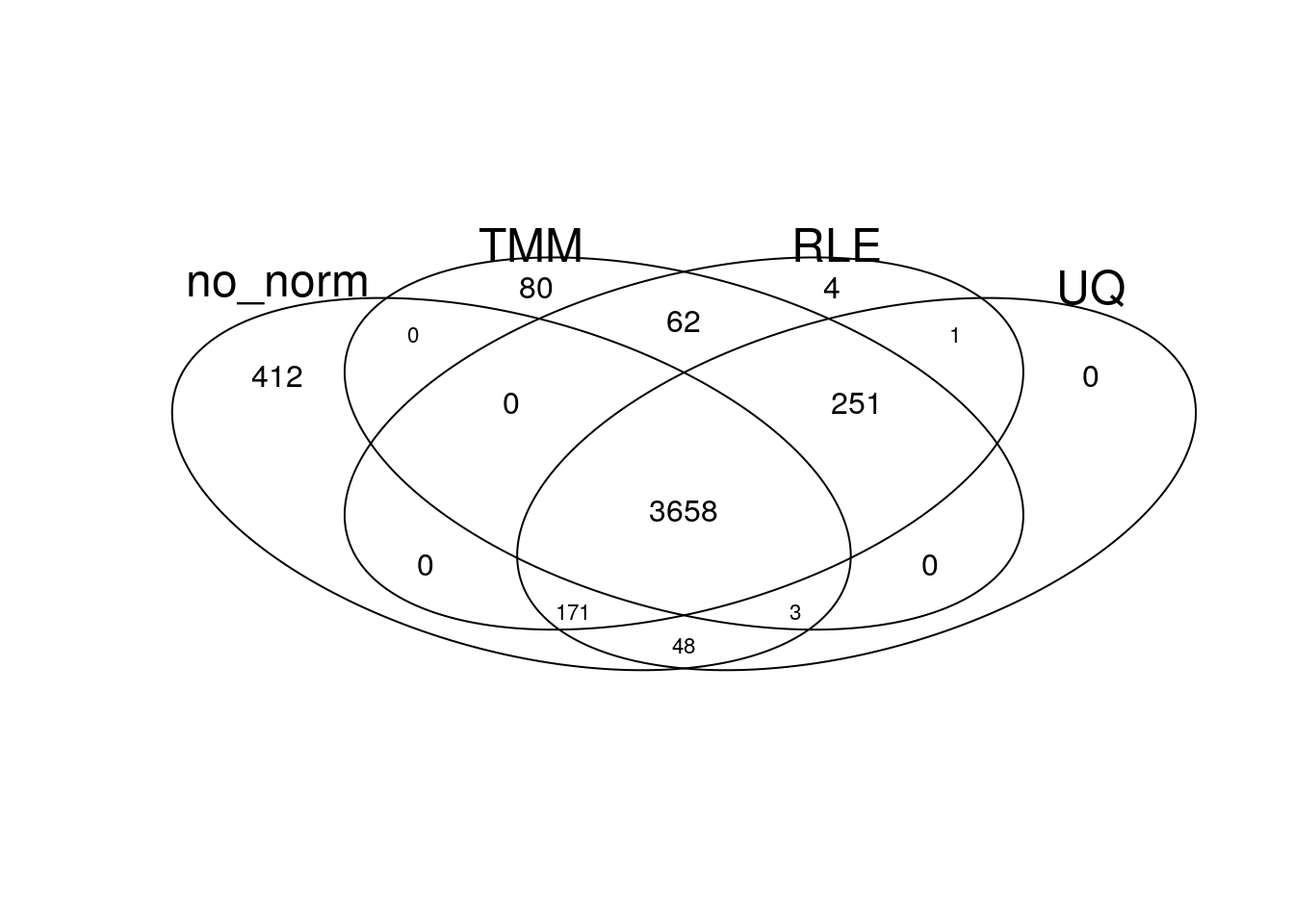
| Version | Author | Date |
|---|---|---|
| 062a0af | Dave Tang | 2024-07-31 |
There is a large overlap of differentially expressed genes in the different normalisation approaches.
gplots::venn(list(TMM = my_de_tmm, RLE = my_de_rle, UQ = my_de_uq))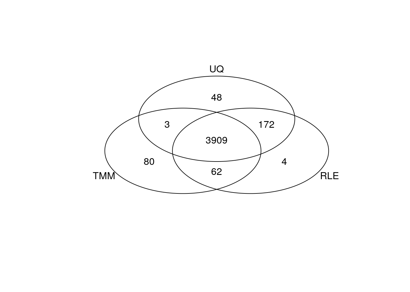
| Version | Author | Date |
|---|---|---|
| 062a0af | Dave Tang | 2024-07-31 |
Data from {pascilla}
Example dataset in the experiment data package {pasilla}.
fn <- system.file("extdata", "pasilla_gene_counts.tsv", package = "pasilla", mustWork = TRUE)
counts <- as.matrix(read.csv(fn, sep="\t", row.names = "gene_id"))
head(counts)
untreated1 untreated2 untreated3 untreated4 treated1 treated2
FBgn0000003 0 0 0 0 0 0
FBgn0000008 92 161 76 70 140 88
FBgn0000014 5 1 0 0 4 0
FBgn0000015 0 2 1 2 1 0
FBgn0000017 4664 8714 3564 3150 6205 3072
FBgn0000018 583 761 245 310 722 299
treated3
FBgn0000003 1
FBgn0000008 70
FBgn0000014 0
FBgn0000015 0
FBgn0000017 3334
FBgn0000018 308Subset counts.
counts_subset <- counts[, c(1,5)]
head(counts_subset)
untreated1 treated1
FBgn0000003 0 0
FBgn0000008 92 140
FBgn0000014 5 4
FBgn0000015 0 1
FBgn0000017 4664 6205
FBgn0000018 583 722Create DGEList object.
group <- factor(colnames(counts_subset))
d <- DGEList(counts=counts_subset, group=group)
d
An object of class "DGEList"
$counts
untreated1 treated1
FBgn0000003 0 0
FBgn0000008 92 140
FBgn0000014 5 4
FBgn0000015 0 1
FBgn0000017 4664 6205
14594 more rows ...
$samples
group lib.size norm.factors
untreated1 untreated1 13972512 1
treated1 treated1 18670279 1Normalise.
d_tmm <- normLibSizes(d, method="TMM")
d_tmm
An object of class "DGEList"
$counts
untreated1 treated1
FBgn0000003 0 0
FBgn0000008 92 140
FBgn0000014 5 4
FBgn0000015 0 1
FBgn0000017 4664 6205
14594 more rows ...
$samples
group lib.size norm.factors
untreated1 untreated1 13972512 0.9639914
treated1 treated1 18670279 1.0373536Summary
The normalisation factors were quite similar between all normalisation methods, which is why the results of the differential expression were quite concordant. Most methods down sized the DHT samples with a normalisation factor of less than one to account for the larger library sizes of these samples.
sessionInfo()R version 4.4.0 (2024-04-24)
Platform: x86_64-pc-linux-gnu
Running under: Ubuntu 22.04.4 LTS
Matrix products: default
BLAS: /usr/lib/x86_64-linux-gnu/openblas-pthread/libblas.so.3
LAPACK: /usr/lib/x86_64-linux-gnu/openblas-pthread/libopenblasp-r0.3.20.so; LAPACK version 3.10.0
locale:
[1] LC_CTYPE=en_US.UTF-8 LC_NUMERIC=C
[3] LC_TIME=en_US.UTF-8 LC_COLLATE=en_US.UTF-8
[5] LC_MONETARY=en_US.UTF-8 LC_MESSAGES=en_US.UTF-8
[7] LC_PAPER=en_US.UTF-8 LC_NAME=C
[9] LC_ADDRESS=C LC_TELEPHONE=C
[11] LC_MEASUREMENT=en_US.UTF-8 LC_IDENTIFICATION=C
time zone: Etc/UTC
tzcode source: system (glibc)
attached base packages:
[1] stats graphics grDevices utils datasets methods base
other attached packages:
[1] gplots_3.1.3.1 edgeR_4.2.1 limma_3.60.4 lubridate_1.9.3
[5] forcats_1.0.0 stringr_1.5.1 dplyr_1.1.4 purrr_1.0.2
[9] readr_2.1.5 tidyr_1.3.1 tibble_3.2.1 ggplot2_3.5.1
[13] tidyverse_2.0.0 workflowr_1.7.1
loaded via a namespace (and not attached):
[1] gtable_0.3.5 xfun_0.44 bslib_0.7.0 caTools_1.18.2
[5] processx_3.8.4 lattice_0.22-6 callr_3.7.6 tzdb_0.4.0
[9] vctrs_0.6.5 tools_4.4.0 ps_1.7.6 bitops_1.0-7
[13] generics_0.1.3 fansi_1.0.6 highr_0.11 pkgconfig_2.0.3
[17] KernSmooth_2.23-22 lifecycle_1.0.4 compiler_4.4.0 git2r_0.33.0
[21] statmod_1.5.0 munsell_0.5.1 getPass_0.2-4 httpuv_1.6.15
[25] htmltools_0.5.8.1 sass_0.4.9 yaml_2.3.8 later_1.3.2
[29] pillar_1.9.0 jquerylib_0.1.4 whisker_0.4.1 cachem_1.1.0
[33] gtools_3.9.5 tidyselect_1.2.1 locfit_1.5-9.9 digest_0.6.35
[37] stringi_1.8.4 splines_4.4.0 rprojroot_2.0.4 fastmap_1.2.0
[41] grid_4.4.0 colorspace_2.1-0 cli_3.6.2 magrittr_2.0.3
[45] utf8_1.2.4 withr_3.0.0 scales_1.3.0 promises_1.3.0
[49] timechange_0.3.0 rmarkdown_2.27 httr_1.4.7 hms_1.1.3
[53] evaluate_0.24.0 knitr_1.47 rlang_1.1.4 Rcpp_1.0.12
[57] glue_1.7.0 rstudioapi_0.16.0 jsonlite_1.8.8 R6_2.5.1
[61] fs_1.6.4