Last updated: 2026-03-24

Checks: 7 0

Knit directory: muse/

This reproducible R Markdown analysis was created with workflowr (version 1.7.2). The Checks tab describes the reproducibility checks that were applied when the results were created. The Past versions tab lists the development history.

R Markdown file: up-to-date

Great! Since the R Markdown file has been committed to the Git repository, you know the exact version of the code that produced these results.

Environment: empty

Great job! The global environment was empty. Objects defined in the global environment can affect the analysis in your R Markdown file in unknown ways. For reproduciblity it’s best to always run the code in an empty environment.

Seed: set.seed(20200712)

The command set.seed(20200712) was run prior to running the code in the R Markdown file. Setting a seed ensures that any results that rely on randomness, e.g. subsampling or permutations, are reproducible.

Session information: recorded

Great job! Recording the operating system, R version, and package versions is critical for reproducibility.

Cache: none

Nice! There were no cached chunks for this analysis, so you can be confident that you successfully produced the results during this run.

File paths: relative

Great job! Using relative paths to the files within your workflowr project makes it easier to run your code on other machines.

Repository version: a46f57c

Great! You are using Git for version control. Tracking code development and connecting the code version to the results is critical for reproducibility.

The results in this page were generated with repository version a46f57c. See the Past versions tab to see a history of the changes made to the R Markdown and HTML files.

Note that you need to be careful to ensure that all relevant files for the analysis have been committed to Git prior to generating the results (you can use wflow_publish or wflow_git_commit). workflowr only checks the R Markdown file, but you know if there are other scripts or data files that it depends on. Below is the status of the Git repository when the results were generated:


Ignored files:
    Ignored:    .Rproj.user/
    Ignored:    data/1M_neurons_filtered_gene_bc_matrices_h5.h5
    Ignored:    data/293t/
    Ignored:    data/293t_3t3_filtered_gene_bc_matrices.tar.gz
    Ignored:    data/293t_filtered_gene_bc_matrices.tar.gz
    Ignored:    data/5k_Human_Donor1_PBMC_3p_gem-x_5k_Human_Donor1_PBMC_3p_gem-x_count_sample_filtered_feature_bc_matrix.h5
    Ignored:    data/5k_Human_Donor2_PBMC_3p_gem-x_5k_Human_Donor2_PBMC_3p_gem-x_count_sample_filtered_feature_bc_matrix.h5
    Ignored:    data/5k_Human_Donor3_PBMC_3p_gem-x_5k_Human_Donor3_PBMC_3p_gem-x_count_sample_filtered_feature_bc_matrix.h5
    Ignored:    data/5k_Human_Donor4_PBMC_3p_gem-x_5k_Human_Donor4_PBMC_3p_gem-x_count_sample_filtered_feature_bc_matrix.h5
    Ignored:    data/97516b79-8d08-46a6-b329-5d0a25b0be98.h5ad
    Ignored:    data/Parent_SC3v3_Human_Glioblastoma_filtered_feature_bc_matrix.tar.gz
    Ignored:    data/brain_counts/
    Ignored:    data/cl.obo
    Ignored:    data/cl.owl
    Ignored:    data/jurkat/
    Ignored:    data/jurkat:293t_50:50_filtered_gene_bc_matrices.tar.gz
    Ignored:    data/jurkat_293t/
    Ignored:    data/jurkat_filtered_gene_bc_matrices.tar.gz
    Ignored:    data/pbmc20k/
    Ignored:    data/pbmc20k_seurat/
    Ignored:    data/pbmc3k.csv
    Ignored:    data/pbmc3k.csv.gz
    Ignored:    data/pbmc3k.h5ad
    Ignored:    data/pbmc3k/
    Ignored:    data/pbmc3k_bpcells_mat/
    Ignored:    data/pbmc3k_export.mtx
    Ignored:    data/pbmc3k_matrix.mtx
    Ignored:    data/pbmc3k_seurat.rds
    Ignored:    data/pbmc4k_filtered_gene_bc_matrices.tar.gz
    Ignored:    data/pbmc_1k_v3_filtered_feature_bc_matrix.h5
    Ignored:    data/pbmc_1k_v3_raw_feature_bc_matrix.h5
    Ignored:    data/refdata-gex-GRCh38-2020-A.tar.gz
    Ignored:    data/seurat_1m_neuron.rds
    Ignored:    data/t_3k_filtered_gene_bc_matrices.tar.gz
    Ignored:    r_packages_4.5.2/

Untracked files:
    Untracked:  .claude/
    Untracked:  CLAUDE.md
    Untracked:  analysis/.claude/
    Untracked:  analysis/aucc.Rmd
    Untracked:  analysis/bimodal.Rmd
    Untracked:  analysis/bioc.Rmd
    Untracked:  analysis/bioc_scrnaseq.Rmd
    Untracked:  analysis/chick_weight.Rmd
    Untracked:  analysis/likelihood.Rmd
    Untracked:  analysis/modelling.Rmd
    Untracked:  analysis/wordpress_readability.Rmd
    Untracked:  bpcells_matrix/
    Untracked:  data/Caenorhabditis_elegans.WBcel235.113.gtf.gz
    Untracked:  data/GCF_043380555.1-RS_2024_12_gene_ontology.gaf.gz
    Untracked:  data/SeuratObj.rds
    Untracked:  data/arab.rds
    Untracked:  data/astronomicalunit.csv
    Untracked:  data/davetang039sblog.WordPress.2026-02-12.xml
    Untracked:  data/femaleMiceWeights.csv
    Untracked:  data/lung_bcell.rds
    Untracked:  m3/
    Untracked:  women.json

Unstaged changes:
    Modified:   analysis/isoform_switch_analyzer.Rmd
    Modified:   analysis/linear_models.Rmd

Note that any generated files, e.g. HTML, png, CSS, etc., are not included in this status report because it is ok for generated content to have uncommitted changes.

These are the previous versions of the repository in which changes were made to the R Markdown (analysis/em.Rmd) and HTML (docs/em.html) files. If you’ve configured a remote Git repository (see ?wflow_git_remote), click on the hyperlinks in the table below to view the files as they were in that past version.

File	Version	Author	Date	Message
Rmd	a46f57c	Dave Tang	2026-03-24	Add background material
html	95b39d2	Dave Tang	2026-03-24	Build site.
Rmd	d7f7bfb	Dave Tang	2026-03-24	Use simulated data for the two-coin example
html	54767a7	Dave Tang	2026-03-23	Build site.
Rmd	7753a73	Dave Tang	2026-03-23	Grading example made concrete
html	ab2ee65	Dave Tang	2026-03-23	Build site.
Rmd	15275c4	Dave Tang	2026-03-23	The EM algorithm

library(ggplot2)

Introduction

The Expectation-Maximisation (EM) algorithm is one of the most widely used tools in statistics and machine learning. It shows up in Gaussian mixture models, hidden Markov models, missing-data problems, and many other settings. But most explanations of EM jump into abstract notation very quickly, which makes it feel more complicated than it actually is.

The core idea is simple. EM is for situations where you are trying to estimate something, but there is hidden information that, if you knew it, would make the problem easy. Since you don’t know the hidden information, you alternate between:

Guessing the hidden information (using your current parameter estimates).
Updating the parameter estimates (using your guesses of the hidden information).

Repeat until things stabilise. That’s it. The rest of this article is about building solid intuition for what this means and why it works.

An Everyday Analogy

Imagine you are a teacher with two teaching assistants, Alice and Bob, who grade homework. You receive a stack of graded assignments but their names have fallen off — you can see the scores each student received, but you do not know which TA graded which assignment.

You want to figure out each TA’s grading tendency (say, the average score they give). If you knew who graded each assignment, this would be trivial: split the assignments into two piles and compute the average for each pile.

But you don’t know who graded what. So you do the following:

Start with a guess: maybe Alice grades generously (average ~85) and Bob grades strictly (average ~70).
E-step: For each assignment, ask: “Given these guessed averages, which TA probably graded this one?” An assignment with a score of 90 is more likely from Alice; a score of 65 is more likely from Bob. A score of 78 could go either way, so you assign partial credit — maybe 60% chance Alice, 40% chance Bob.
M-step: Using these soft assignments, recompute the averages. Alice’s new average is the weighted mean of all scores, weighted by how likely she was to have graded each one. Same for Bob.
Repeat steps 2 and 3 until the averages stop changing.

That is the EM algorithm. The hidden information is “who graded what”, and the parameters are the grading averages.

The Two-Coin Problem

The classic teaching example for EM involves two coins. This problem is small enough to work through by hand, which makes the mechanics completely transparent.

Setup

You have two coins, A and B, with unknown probabilities of landing heads:

Coin A lands heads with probability \(\theta_A\) (unknown).
Coin B lands heads with probability \(\theta_B\) (unknown).

Someone runs several rounds of an experiment. In each round, they secretly pick one of the two coins (you don’t know which), flip it 10 times, and tell you how many heads came up. Your job: estimate \(\theta_A\) and \(\theta_B\).

Let’s simulate this. We’ll set the true biases to \(\theta_A = 0.8\) and \(\theta_B = 0.3\), generate the data, and then see how close EM can get — pretending we don’t know the true values.

set.seed(1984)

# True (hidden) parameters
true_theta_A <- 0.8
true_theta_B <- 0.3

# Simulate 10 rounds: randomly pick a coin, flip it 10 times
n_rounds <- 10
n_flips <- 10

coin_used <- sample(c("A", "B"), n_rounds, replace = TRUE)
heads <- ifelse(
  coin_used == "A",
  rbinom(n_rounds, size = n_flips, prob = true_theta_A),
  rbinom(n_rounds, size = n_flips, prob = true_theta_B)
)

Here is what the experimenter tells us — just the number of heads per round. The coin column is hidden from us.

data.frame(
  Round = seq_len(n_rounds),
  Heads = heads,
  Coin_used = paste0(coin_used, " (hidden)")
)

   Round Heads  Coin_used
1      1     3 B (hidden)
2      2     0 B (hidden)
3      3     3 B (hidden)
4      4     5 B (hidden)
5      5     9 A (hidden)
6      6    10 A (hidden)
7      7     4 B (hidden)
8      8     3 B (hidden)
9      9     6 A (hidden)
10    10     9 A (hidden)

If we knew the hidden column, we could just compute the proportion of heads for each coin. Since we don’t, we use EM.

Step by Step

Before we look at the code, let’s unpack the key ideas that the E-step and M-step rely on.

Probability vs Likelihood

These two words sound interchangeable, but they ask different questions:

Probability asks: given that I know the coin has bias \(\theta = 0.8\), what is the chance of seeing 7 heads in 10 flips? The parameter is fixed and we are asking about the data.
Likelihood asks: given that I observed 7 heads in 10 flips, how plausible is it that the coin has bias \(\theta = 0.8\)? The data is fixed and we are asking about the parameter.

Mathematically, the same formula is used for both — the binomial probability mass function dbinom(). The difference is in what we treat as known and what we treat as unknown. When we hold the data fixed and vary the parameter, we call the result the likelihood.

Conditional Probability and Bayes’ Rule

In the E-step, we need to answer: “Given the heads count in this round and our current guesses for \(\theta_A\) and \(\theta_B\), what is the probability that coin A was used?” This is a conditional probability — the probability of one event (coin A was used) given that another event has occurred (we observed a specific number of heads).

Bayes’ rule gives us the answer:

\[P(\text{coin A} \mid \text{data}) = \frac{P(\text{data} \mid \text{coin A}) \times P(\text{coin A})}{P(\text{data} \mid \text{coin A}) \times P(\text{coin A}) + P(\text{data} \mid \text{coin B}) \times P(\text{coin B})}\]

Breaking this down:

\(P(\text{data} \mid \text{coin A})\) is the likelihood: how probable is this round’s outcome if coin A was used? We compute this with dbinom(heads, size = n_flips, prob = theta_A).
\(P(\text{coin A})\) is the prior: before looking at the data, how likely is it that coin A was picked? We assume each coin is equally likely, so \(P(\text{coin A}) = P(\text{coin B}) = 0.5\). Because the priors are equal, they cancel out and the formula simplifies to:

\[P(\text{coin A} \mid \text{data}) = \frac{P(\text{data} \mid \text{coin A})}{P(\text{data} \mid \text{coin A}) + P(\text{data} \mid \text{coin B})}\]

This is just “coin A’s likelihood divided by the total likelihood”. If coin A makes the observed data twice as likely as coin B, then coin A gets twice the credit.

Responsibility

The result of this calculation — \(P(\text{coin A} \mid \text{data})\) — is called the responsibility. It is a number between 0 and 1 for each round. A responsibility of 0.9 for coin A means: “given our current parameter guesses, we are 90% confident coin A was used in this round.”

The Weighted Update (M-step)

Once we have responsibilities, we update the bias estimates. The M-step computes:

\[\theta_A^{\text{new}} = \frac{\sum_{i} r_{A,i} \times h_i}{\sum_{i} r_{A,i} \times n}\]

where \(r_{A,i}\) is the responsibility of coin A for round \(i\), \(h_i\) is the number of heads, and \(n\) is the number of flips per round.

What does this mean? Consider two extremes:

If \(r_{A,i} = 1\) for some rounds and 0 for others, this becomes the ordinary proportion of heads across only the rounds assigned to coin A. This is what you would compute if you knew the labels.
If \(r_{A,i} = 0.7\) for a round, that round contributes to coin A’s estimate with 70% weight and to coin B’s with 30%. Each round “splits” its evidence between the two coins according to how likely each coin was.

In this way, the responsibilities act as soft labels: instead of assigning each round to exactly one coin, they spread each round’s data proportionally across both coins.

Initial Guess

We need a starting point. Let’s guess \(\theta_A = 0.6\) and \(\theta_B = 0.5\).

# EM for the two-coin problem
em_two_coins <- function(heads, n_flips, theta_A_init, theta_B_init,
                         max_iter = 20, tol = 1e-6) {

  theta_A <- theta_A_init
  theta_B <- theta_B_init
  n_rounds <- length(heads)
  history <- data.frame(
    iteration = integer(),
    theta_A = numeric(),
    theta_B = numeric()
  )
  history <- rbind(history, data.frame(
    iteration = 0, theta_A = theta_A, theta_B = theta_B
  ))

  for (iter in seq_len(max_iter)) {
    # --- E-step ---
    # For each round, compute the probability that coin A was used
    # P(coin A | data) is proportional to P(data | coin A) * P(coin A)
    # Assume equal prior: P(coin A) = P(coin B) = 0.5

    # Likelihood of observing the data under each coin (binomial)
    lik_A <- dbinom(heads, size = n_flips, prob = theta_A)
    lik_B <- dbinom(heads, size = n_flips, prob = theta_B)

    # Responsibility: probability that coin A generated each round
    resp_A <- lik_A / (lik_A + lik_B)
    resp_B <- 1 - resp_A

    # --- M-step ---
    # Update theta_A: weighted average of head proportions, weighted by resp_A
    theta_A_new <- sum(resp_A * heads) / sum(resp_A * n_flips)
    theta_B_new <- sum(resp_B * heads) / sum(resp_B * n_flips)

    history <- rbind(history, data.frame(
      iteration = iter, theta_A = theta_A_new, theta_B = theta_B_new
    ))

    # Check convergence
    if (abs(theta_A_new - theta_A) < tol && abs(theta_B_new - theta_B) < tol) {
      theta_A <- theta_A_new
      theta_B <- theta_B_new
      break
    }

    theta_A <- theta_A_new
    theta_B <- theta_B_new
  }

  list(
    theta_A = theta_A,
    theta_B = theta_B,
    iterations = iter,
    history = history
  )
}

result <- em_two_coins(heads, n_flips,
                       theta_A_init = 0.6, theta_B_init = 0.5)

cat(sprintf("Converged in %d iterations\n\n", result$iterations))

Converged in 16 iterations

cat(sprintf("  Estimated: theta_A = %.4f   True: %.4f\n", result$theta_A, true_theta_A))

  Estimated: theta_A = 0.9266   True: 0.8000

cat(sprintf("  Estimated: theta_B = %.4f   True: %.4f\n", result$theta_B, true_theta_B))

  Estimated: theta_B = 0.3408   True: 0.3000

With only 10 rounds of data, the estimates may not be perfect — but they should be in the right ballpark. EM correctly identifies which coin is biased toward heads and which toward tails.

What Happened at Each Iteration

Let’s look at the first few iterations in detail to see the E-step and M-step playing out.

# Show detailed E-step and M-step for the first 3 iterations
theta_A <- 0.6
theta_B <- 0.5

for (iter in 1:3) {
  cat(sprintf("=== Iteration %d ===\n", iter))
  cat(sprintf("Current guesses: theta_A = %.4f, theta_B = %.4f\n\n", theta_A, theta_B))

  lik_A <- dbinom(heads, size = n_flips, prob = theta_A)
  lik_B <- dbinom(heads, size = n_flips, prob = theta_B)
  resp_A <- lik_A / (lik_A + lik_B)

  cat("E-step — responsibility of coin A for each round:\n")
  for (i in seq_along(heads)) {
    cat(sprintf("  Round %d (%d heads): P(coin A) = %.3f, P(coin B) = %.3f\n",
                i, heads[i], resp_A[i], 1 - resp_A[i]))
  }

  theta_A <- sum(resp_A * heads) / sum(resp_A * n_flips)
  theta_B <- sum((1 - resp_A) * heads) / sum((1 - resp_A) * n_flips)

  cat(sprintf("\nM-step — updated estimates: theta_A = %.4f, theta_B = %.4f\n\n", theta_A, theta_B))
}

=== Iteration 1 ===
Current guesses: theta_A = 0.6000, theta_B = 0.5000

E-step — responsibility of coin A for each round:
  Round 1 (3 heads): P(coin A) = 0.266, P(coin B) = 0.734
  Round 2 (0 heads): P(coin A) = 0.097, P(coin B) = 0.903
  Round 3 (3 heads): P(coin A) = 0.266, P(coin B) = 0.734
  Round 4 (5 heads): P(coin A) = 0.449, P(coin B) = 0.551
  Round 5 (9 heads): P(coin A) = 0.805, P(coin B) = 0.195
  Round 6 (10 heads): P(coin A) = 0.861, P(coin B) = 0.139
  Round 7 (4 heads): P(coin A) = 0.352, P(coin B) = 0.648
  Round 8 (3 heads): P(coin A) = 0.266, P(coin B) = 0.734
  Round 9 (6 heads): P(coin A) = 0.550, P(coin B) = 0.450
  Round 10 (9 heads): P(coin A) = 0.805, P(coin B) = 0.195

M-step — updated estimates: theta_A = 0.6879, theta_B = 0.3701

=== Iteration 2 ===
Current guesses: theta_A = 0.6879, theta_B = 0.3701

E-step — responsibility of coin A for each round:
  Round 1 (3 heads): P(coin A) = 0.045, P(coin B) = 0.955
  Round 2 (0 heads): P(coin A) = 0.001, P(coin B) = 0.999
  Round 3 (3 heads): P(coin A) = 0.045, P(coin B) = 0.955
  Round 4 (5 heads): P(coin A) = 0.399, P(coin B) = 0.601
  Round 5 (9 heads): P(coin A) = 0.992, P(coin B) = 0.008
  Round 6 (10 heads): P(coin A) = 0.998, P(coin B) = 0.002
  Round 7 (4 heads): P(coin A) = 0.150, P(coin B) = 0.850
  Round 8 (3 heads): P(coin A) = 0.045, P(coin B) = 0.955
  Round 9 (6 heads): P(coin A) = 0.713, P(coin B) = 0.287
  Round 10 (9 heads): P(coin A) = 0.992, P(coin B) = 0.008

M-step — updated estimates: theta_A = 0.8017, theta_B = 0.3004

=== Iteration 3 ===
Current guesses: theta_A = 0.8017, theta_B = 0.3004

E-step — responsibility of coin A for each round:
  Round 1 (3 heads): P(coin A) = 0.003, P(coin B) = 0.997
  Round 2 (0 heads): P(coin A) = 0.000, P(coin B) = 1.000
  Round 3 (3 heads): P(coin A) = 0.003, P(coin B) = 0.997
  Round 4 (5 heads): P(coin A) = 0.198, P(coin B) = 0.802
  Round 5 (9 heads): P(coin A) = 0.999, P(coin B) = 0.001
  Round 6 (10 heads): P(coin A) = 1.000, P(coin B) = 0.000
  Round 7 (4 heads): P(coin A) = 0.026, P(coin B) = 0.974
  Round 8 (3 heads): P(coin A) = 0.003, P(coin B) = 0.997
  Round 9 (6 heads): P(coin A) = 0.700, P(coin B) = 0.300
  Round 10 (9 heads): P(coin A) = 0.999, P(coin B) = 0.001

M-step — updated estimates: theta_A = 0.8473, theta_B = 0.3080

Notice how the responsibilities shift over iterations. In the beginning, the guesses are close together so the model is unsure which coin generated which round. As the estimates improve, the model becomes more confident: rounds with many heads are assigned more strongly to the higher-probability coin and vice versa.

Convergence Plot

history_long <- data.frame(
  iteration = rep(result$history$iteration, 2),
  theta = c(result$history$theta_A, result$history$theta_B),
  coin = rep(c("Coin A", "Coin B"), each = nrow(result$history))
)

ggplot(history_long, aes(x = iteration, y = theta, colour = coin)) +
  geom_line(linewidth = 1) +
  geom_point(size = 2) +
  geom_hline(yintercept = true_theta_A, linetype = "dashed", colour = "grey40") +
  geom_hline(yintercept = true_theta_B, linetype = "dashed", colour = "grey40") +
  annotate("text", x = max(history_long$iteration), y = true_theta_A + 0.03,
           label = paste0("True theta_A = ", true_theta_A),
           hjust = 1, colour = "grey40") +
  annotate("text", x = max(history_long$iteration), y = true_theta_B - 0.03,
           label = paste0("True theta_B = ", true_theta_B),
           hjust = 1, colour = "grey40") +
  labs(x = "Iteration", y = "Estimated Bias (probability of heads)",
       colour = "", title = "EM convergence for the two-coin problem") +
  theme_minimal()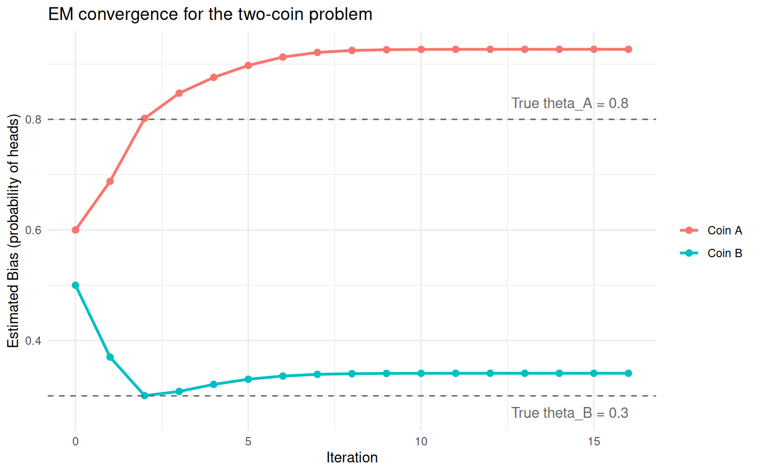

Convergence of coin bias estimates across EM iterations. Dashed lines show the true values.

Version	Author	Date
95b39d2	Dave Tang	2026-03-24
ab2ee65	Dave Tang	2026-03-23

The two estimates start close together and gradually separate as the algorithm figures out which rounds go with which coin. The dashed lines show the true biases we used to simulate the data.

More Data, Better Estimates

With only 10 rounds, the estimates are reasonable but not exact. What happens if we give EM more data? Just as you would get a better estimate of a coin’s bias by flipping it more times, EM gets closer to the truth with more rounds.

round_sizes <- c(10, 25, 50, 100, 250, 500)
n_reps <- 50  # repeat each size to show variability

sim_results <- do.call(rbind, lapply(round_sizes, function(nr) {
  do.call(rbind, lapply(seq_len(n_reps), function(rep) {
    coin <- sample(c("A", "B"), nr, replace = TRUE)
    h <- ifelse(
      coin == "A",
      rbinom(nr, size = n_flips, prob = true_theta_A),
      rbinom(nr, size = n_flips, prob = true_theta_B)
    )
    fit <- em_two_coins(h, n_flips, theta_A_init = 0.6, theta_B_init = 0.5)

    # EM may swap the labels — assign higher estimate to coin A
    tA <- max(fit$theta_A, fit$theta_B)
    tB <- min(fit$theta_A, fit$theta_B)

    data.frame(n_rounds = nr, rep = rep, theta_A = tA, theta_B = tB)
  }))
}))

sim_long <- data.frame(
  n_rounds = rep(sim_results$n_rounds, 2),
  estimate = c(sim_results$theta_A, sim_results$theta_B),
  coin = rep(c("Coin A", "Coin B"), each = nrow(sim_results))
)

ggplot(sim_long, aes(x = factor(n_rounds), y = estimate, fill = coin)) +
  geom_boxplot(alpha = 0.7, outlier.size = 0.8) +
  geom_hline(yintercept = true_theta_A, linetype = "dashed", colour = "grey30") +
  geom_hline(yintercept = true_theta_B, linetype = "dashed", colour = "grey30") +
  annotate("text", x = 6.4, y = true_theta_A + 0.02,
           label = paste0("True = ", true_theta_A), colour = "grey30", hjust = 1) +
  annotate("text", x = 6.4, y = true_theta_B - 0.02,
           label = paste0("True = ", true_theta_B), colour = "grey30", hjust = 1) +
  labs(x = "Number of Rounds", y = "Estimated Bias",
       fill = "", title = "EM estimates improve with more data") +
  theme_minimal()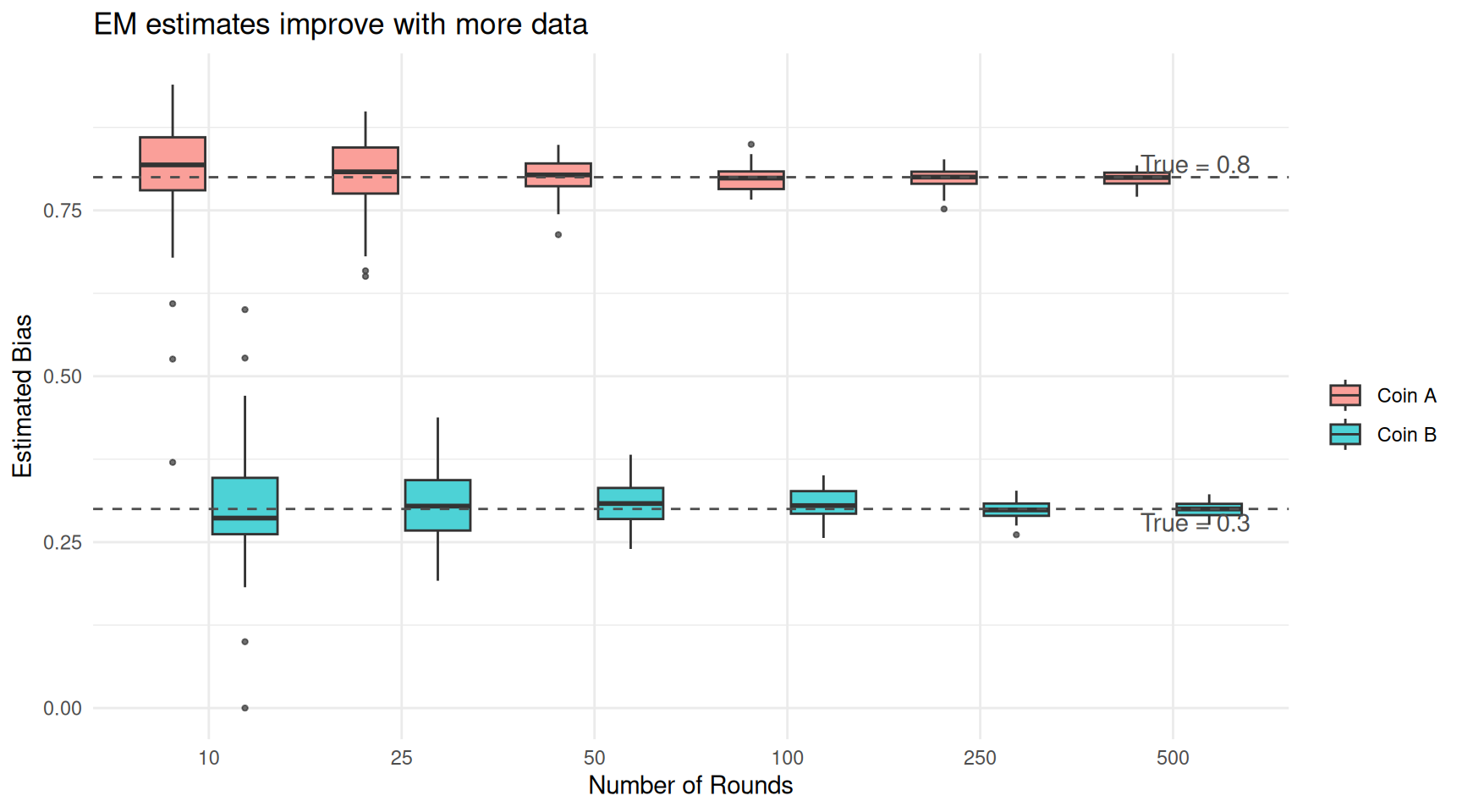

EM estimates improve as the number of rounds increases. With enough data, the estimates converge to the true values.

Version	Author	Date
95b39d2	Dave Tang	2026-03-24

With 10 rounds, the estimates are noisy — each repetition of the experiment gives a somewhat different answer. By 100 rounds, the boxes have tightened considerably. By 500 rounds, the estimates are tightly clustered around the true values. This is a general property: EM is a consistent estimator, meaning it converges to the truth given enough data.

The Grading Example — Made Concrete

Earlier we described a teacher trying to figure out whether Alice or Bob graded each assignment, given only the scores. Let’s turn that analogy into a full worked example with simulated data.

Setting the Scene

Alice is a generous grader — her scores tend to cluster around 82 with some spread. Bob is stricter — his scores cluster around 65. Over the semester, they graded 200 assignments between them (Alice graded about 55%, Bob about 45%). Unfortunately the TA names fell off, so all we have is a pile of 200 scores.

set.seed(1984)

n_alice <- 110
n_bob <- 90

alice_scores <- rnorm(n_alice, mean = 82, sd = 7)
bob_scores <- rnorm(n_bob, mean = 65, sd = 6)

# What we observe: a single pile of scores with no labels
scores <- c(alice_scores, bob_scores)
true_grader <- c(rep("Alice", n_alice), rep("Bob", n_bob))

ggplot(data.frame(score = scores), aes(x = score)) +
  geom_histogram(aes(y = after_stat(density)), bins = 30,
                 fill = "steelblue", colour = "white", alpha = 0.7) +
  geom_density(colour = "red", linewidth = 0.8) +
  labs(x = "Score", y = "Density",
       title = "All 200 assignment scores (grader unknown)") +
  theme_minimal()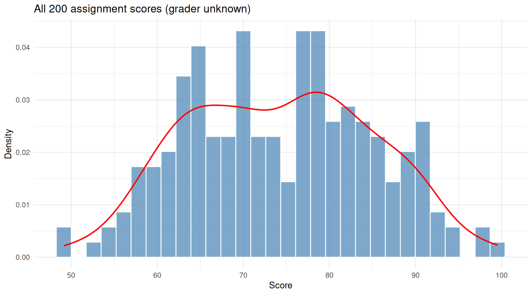

The pile of 200 scores. Two overlapping humps hint at two graders, but we don’t know who graded what.

Version	Author	Date
54767a7	Dave Tang	2026-03-23

The histogram shows a hint of two humps. EM will try to recover the two grading distributions.

Running EM

The parameters we want to estimate are:

\(\mu_A\), \(\sigma_A\): Alice’s average score and spread.
\(\mu_B\), \(\sigma_B\): Bob’s average score and spread.
\(\pi_A\): the proportion of assignments Alice graded (and \(\pi_B = 1 - \pi_A\)).

We start with a rough guess: grader 1 averages around 75 and grader 2 averages around 70 — intentionally mediocre starting values.

em_grading <- function(scores, max_iter = 50, tol = 1e-6) {
  n <- length(scores)

  # Initial guesses (deliberately rough)
  mu <- c(75, 70)
  sigma <- c(10, 10)
  pi_k <- c(0.5, 0.5)

  history <- list()

  for (iter in seq_len(max_iter)) {
    # E-step: for each score, how likely is it from grader 1 vs grader 2?
    lik_1 <- pi_k[1] * dnorm(scores, mean = mu[1], sd = sigma[1])
    lik_2 <- pi_k[2] * dnorm(scores, mean = mu[2], sd = sigma[2])
    resp_1 <- lik_1 / (lik_1 + lik_2)
    resp_2 <- 1 - resp_1

    # M-step: re-estimate parameters using responsibilities as weights
    N_1 <- sum(resp_1)
    N_2 <- sum(resp_2)

    mu_new <- c(sum(resp_1 * scores) / N_1,
                sum(resp_2 * scores) / N_2)
    sigma_new <- c(sqrt(sum(resp_1 * (scores - mu_new[1])^2) / N_1),
                   sqrt(sum(resp_2 * (scores - mu_new[2])^2) / N_2))
    pi_new <- c(N_1 / n, N_2 / n)

    history[[iter]] <- data.frame(
      iteration = iter,
      grader = c("Grader 1", "Grader 2"),
      mu = mu_new,
      sigma = sigma_new,
      weight = pi_new
    )

    if (max(abs(mu_new - mu)) < tol) break
    mu <- mu_new
    sigma <- sigma_new
    pi_k <- pi_new
  }

  list(mu = mu_new, sigma = sigma_new, pi_k = pi_new,
       resp_1 = resp_1, history = do.call(rbind, history),
       iterations = iter)
}

fit_grade <- em_grading(scores)

cat(sprintf("Converged in %d iterations\n\n", fit_grade$iterations))

Converged in 50 iterations

cat("Estimated parameters:\n")

Estimated parameters:

cat(sprintf("  Grader 1: mean = %.1f, sd = %.1f, proportion = %.0f%%\n",
            fit_grade$mu[1], fit_grade$sigma[1], fit_grade$pi_k[1] * 100))

  Grader 1: mean = 81.9, sd = 7.1, proportion = 54%

cat(sprintf("  Grader 2: mean = %.1f, sd = %.1f, proportion = %.0f%%\n",
            fit_grade$mu[2], fit_grade$sigma[2], fit_grade$pi_k[2] * 100))

  Grader 2: mean = 65.2, sd = 6.3, proportion = 46%

cat("\nTrue parameters:\n")


True parameters:

cat(sprintf("  Alice:    mean = 82.0, sd = 7.0, proportion = 55%%\n"))

  Alice:    mean = 82.0, sd = 7.0, proportion = 55%

cat(sprintf("  Bob:      mean = 65.0, sd = 6.0, proportion = 45%%\n"))

  Bob:      mean = 65.0, sd = 6.0, proportion = 45%

EM recovers values close to the truth, despite starting with guesses that were well off.

Watching It Converge

ggplot(fit_grade$history, aes(x = iteration, y = mu, colour = grader)) +
  geom_line(linewidth = 1) +
  geom_point(size = 2) +
  geom_hline(yintercept = 82, linetype = "dashed", colour = "grey40") +
  geom_hline(yintercept = 65, linetype = "dashed", colour = "grey40") +
  annotate("text", x = max(fit_grade$history$iteration), y = 83.5,
           label = "Alice's true mean (82)", hjust = 1, colour = "grey40") +
  annotate("text", x = max(fit_grade$history$iteration), y = 63.5,
           label = "Bob's true mean (65)", hjust = 1, colour = "grey40") +
  labs(x = "Iteration", y = "Estimated Mean Score",
       colour = "", title = "EM convergence for the grading problem") +
  theme_minimal()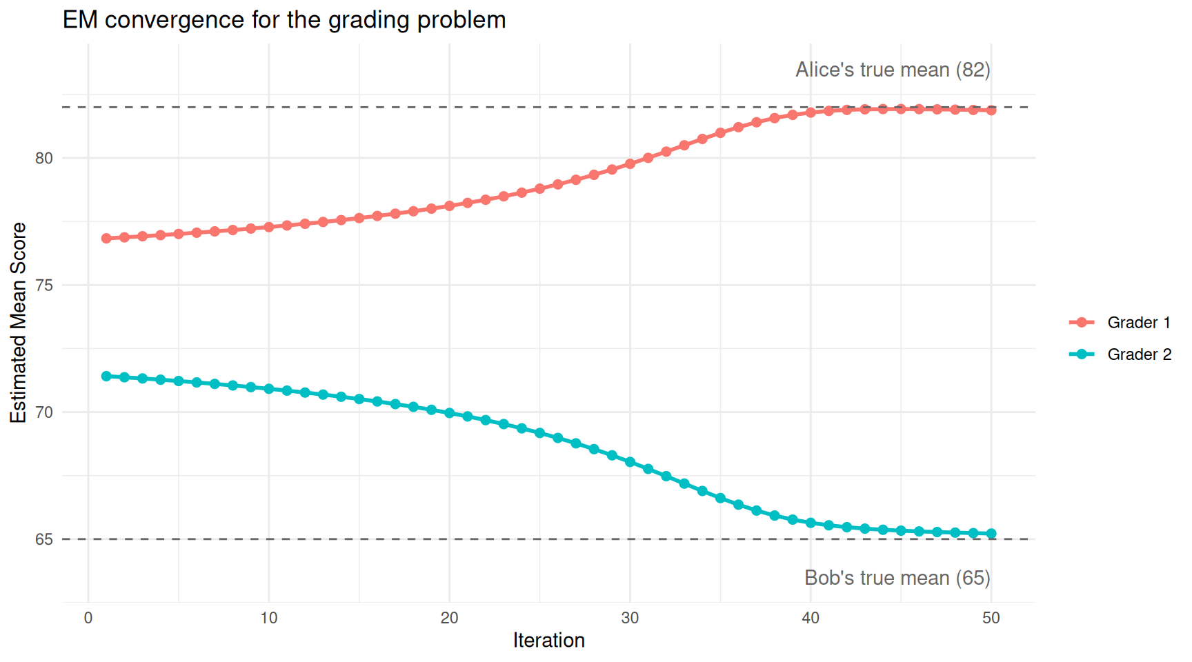

The estimated grading averages converge from the initial guesses (75 and 70) toward the true values.

Version	Author	Date
54767a7	Dave Tang	2026-03-23

The two estimates start close together (75 and 70) and separate rapidly as EM figures out the two grading styles.

Looking at Individual Assignments

After convergence, each assignment has a responsibility — the probability that grader 1 (Alice) gave that score. Let’s look at a few assignments to see how EM reasons about them.

# Pick a few illustrative assignments
examples <- c(
  which.max(scores),                          # highest score
  which.min(scores),                          # lowest score
  which.min(abs(scores - mean(scores)))       # most ambiguous (near overall mean)
)

cat("How EM assigns individual assignments:\n\n")

How EM assigns individual assignments:

for (i in examples) {
  cat(sprintf(
    "  Score = %.1f → P(Alice) = %.1f%%, P(Bob) = %.1f%%  [truly graded by %s]\n",
    scores[i],
    fit_grade$resp_1[i] * 100,
    (1 - fit_grade$resp_1[i]) * 100,
    true_grader[i]
  ))
}

  Score = 99.5 → P(Alice) = 100.0%, P(Bob) = 0.0%  [truly graded by Alice]
  Score = 49.1 → P(Alice) = 0.1%, P(Bob) = 99.9%  [truly graded by Bob]
  Score = 74.2 → P(Alice) = 61.9%, P(Bob) = 38.1%  [truly graded by Alice]

High scores are confidently assigned to Alice (the generous grader), low scores to Bob (the strict grader), and middle scores are genuinely ambiguous.

df_assign <- data.frame(
  score = scores,
  p_alice = fit_grade$resp_1,
  true_grader = true_grader
)

ggplot(df_assign, aes(x = score, y = p_alice, colour = true_grader)) +
  geom_point(alpha = 0.6, size = 2) +
  geom_hline(yintercept = 0.5, linetype = "dashed", colour = "grey50") +
  labs(x = "Score", y = "P(Alice graded this)",
       colour = "True Grader",
       title = "EM's soft assignments vs the truth") +
  theme_minimal()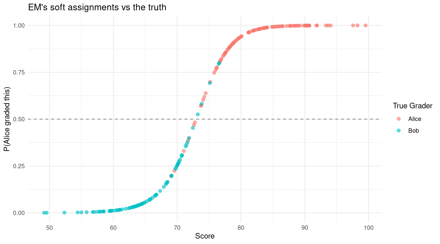

Each assignment coloured by EM’s confidence that Alice graded it. Scores in the overlap region (around 70-75) are genuinely uncertain.

Version	Author	Date
54767a7	Dave Tang	2026-03-23

Points above the dashed line are assigned to Alice; points below to Bob. The colour shows the truth. Most assignments are classified correctly, with mistakes concentrated in the overlap region where the two graders’ score distributions blend together — exactly where you would expect genuine uncertainty.

How Accurate Are the Hard Assignments?

If we assign each paper to whichever grader has the higher responsibility, how often do we get it right?

hard_assignment <- ifelse(fit_grade$resp_1 > 0.5, "Alice", "Bob")
accuracy <- mean(hard_assignment == true_grader)
cat(sprintf("Classification accuracy: %.1f%%\n", accuracy * 100))

Classification accuracy: 93.0%

cat("\nConfusion matrix:\n")


Confusion matrix:

print(table(Predicted = hard_assignment, True = true_grader))

         True
Predicted Alice Bob
    Alice   101   5
    Bob       9  85

The errors are concentrated among scores in the 70–78 range where Alice’s low scores and Bob’s high scores overlap. No method can perfectly separate those, because the data genuinely looks the same regardless of which grader produced it.

EM for Gaussian Mixtures

The two-coin problem illustrates the logic of EM in a discrete setting. The same logic applies to continuous data. The most common application is fitting Gaussian mixture models (GMMs), where you assume your data comes from a blend of several normal (bell-curve) distributions and you want to recover their parameters.

For a detailed treatment of GMMs, see the Gaussian mixture model article. Here we focus on the EM mechanics.

Simulated Data

set.seed(1984)

# Two-component Gaussian mixture
n <- 800
n1 <- round(n * 0.65)
n2 <- n - n1

x <- c(rnorm(n1, mean = 2, sd = 0.8),
       rnorm(n2, mean = 6, sd = 1.0))

true_labels <- c(rep(1, n1), rep(2, n2))

ggplot(data.frame(x = x), aes(x = x)) +
  geom_histogram(aes(y = after_stat(density)), bins = 50,
                 fill = "steelblue", colour = "white", alpha = 0.7) +
  geom_density(colour = "red", linewidth = 0.8) +
  labs(x = "Value", y = "Density",
       title = "Observed data from an unknown mixture") +
  theme_minimal()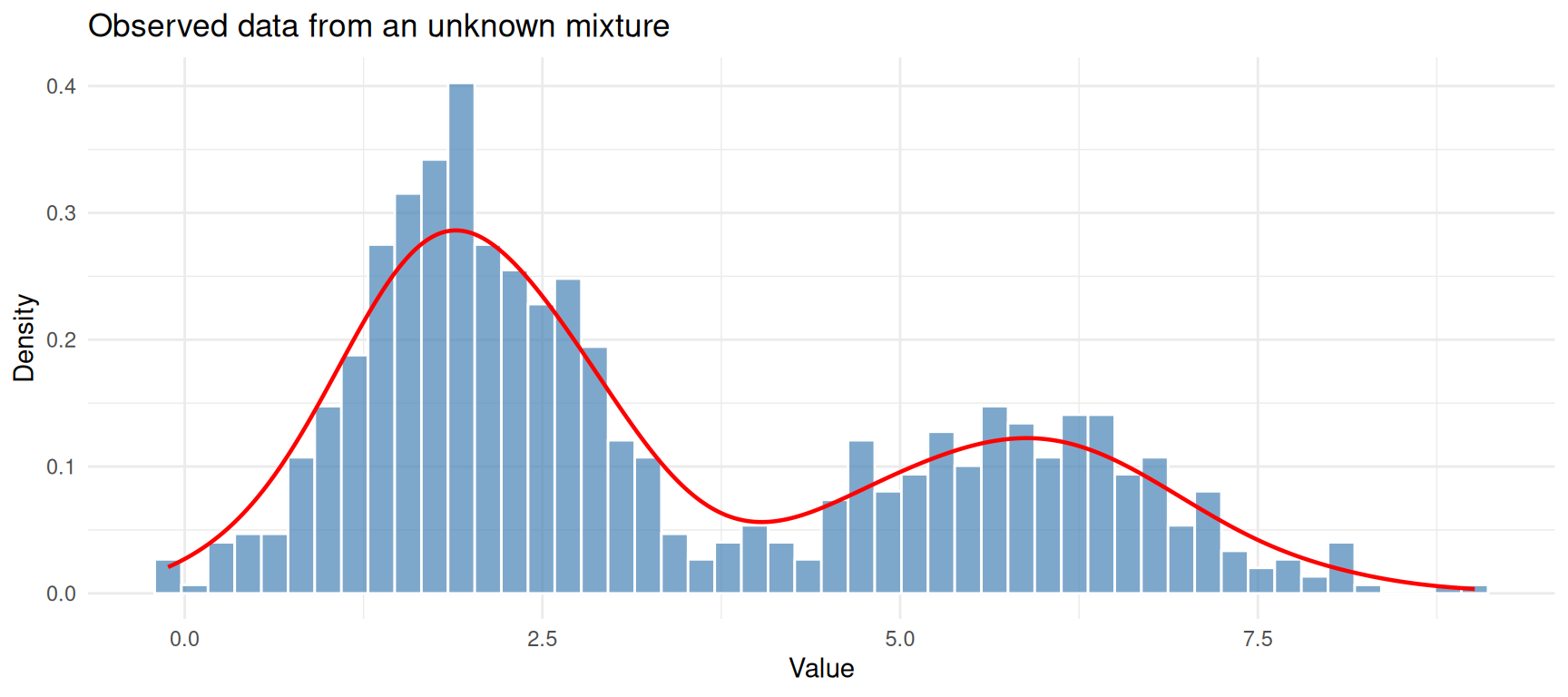

Simulated data from two overlapping Gaussian components.

Version	Author	Date
ab2ee65	Dave Tang	2026-03-23

We know this data was generated by two Gaussians, but we will pretend we don’t and let EM figure it out.

Watching EM Iterate

To see exactly what EM is doing, we’ll record the state at each iteration and plot it.

em_gaussian <- function(x, K = 2, max_iter = 30, tol = 1e-6) {
  n <- length(x)

  # Initialise: spread means across the data range
  mu <- quantile(x, probs = seq(0.3, 0.7, length.out = K))
  sigma <- rep(sd(x), K)
  pi_k <- rep(1 / K, K)

  snapshots <- list()

  for (iter in seq_len(max_iter)) {
    # E-step
    resp <- matrix(0, nrow = n, ncol = K)
    for (k in seq_len(K)) {
      resp[, k] <- pi_k[k] * dnorm(x, mean = mu[k], sd = sigma[k])
    }
    resp <- resp / rowSums(resp)

    # M-step
    N_k <- colSums(resp)
    mu_new <- colSums(resp * x) / N_k
    sigma_new <- sqrt(colSums(resp * outer(x, mu_new, "-")^2) / N_k)
    pi_new <- N_k / n

    # Record snapshot
    snapshots[[iter]] <- list(
      iter = iter, mu = mu_new, sigma = sigma_new,
      pi_k = pi_new, resp = resp
    )

    if (max(abs(mu_new - mu)) < tol) break
    mu <- mu_new
    sigma <- sigma_new
    pi_k <- pi_new
  }

  list(mu = mu_new, sigma = sigma_new, pi_k = pi_new,
       resp = resp, snapshots = snapshots, iterations = iter)
}

fit <- em_gaussian(x, K = 2)
cat(sprintf("Converged in %d iterations\n\n", fit$iterations))

Converged in 30 iterations

cat(sprintf("Component 1: mean = %.2f, sd = %.2f, weight = %.2f\n",
            fit$mu[1], fit$sigma[1], fit$pi_k[1]))

Component 1: mean = 1.95, sd = 0.76, weight = 0.64

cat(sprintf("Component 2: mean = %.2f, sd = %.2f, weight = %.2f\n",
            fit$mu[2], fit$sigma[2], fit$pi_k[2]))

Component 2: mean = 5.83, sd = 1.06, weight = 0.36

# Select a few iterations to visualise
show_iters <- c(1, 3, 5, fit$iterations)
show_iters <- unique(pmin(show_iters, fit$iterations))

x_grid <- seq(min(x) - 1, max(x) + 1, length.out = 500)

plot_data <- do.call(rbind, lapply(show_iters, function(i) {
  s <- fit$snapshots[[i]]
  data.frame(
    x = rep(x_grid, 3),
    density = c(
      s$pi_k[1] * dnorm(x_grid, s$mu[1], s$sigma[1]),
      s$pi_k[2] * dnorm(x_grid, s$mu[2], s$sigma[2]),
      s$pi_k[1] * dnorm(x_grid, s$mu[1], s$sigma[1]) +
        s$pi_k[2] * dnorm(x_grid, s$mu[2], s$sigma[2])
    ),
    curve = rep(c("Component 1", "Component 2", "Mixture"), each = length(x_grid)),
    iteration = paste("Iteration", i)
  )
}))

plot_data$iteration <- factor(plot_data$iteration,
                              levels = paste("Iteration", show_iters))

ggplot() +
  geom_histogram(data = data.frame(x = x), aes(x = x, y = after_stat(density)),
                 bins = 50, fill = "grey80", colour = "white") +
  geom_line(data = plot_data, aes(x = x, y = density, colour = curve),
            linewidth = 0.9) +
  scale_colour_manual(values = c("Component 1" = "#E69F00",
                                  "Component 2" = "#56B4E9",
                                  "Mixture" = "red")) +
  facet_wrap(~iteration, ncol = 2) +
  labs(x = "Value", y = "Density", colour = "",
       title = "EM algorithm iteration by iteration") +
  theme_minimal()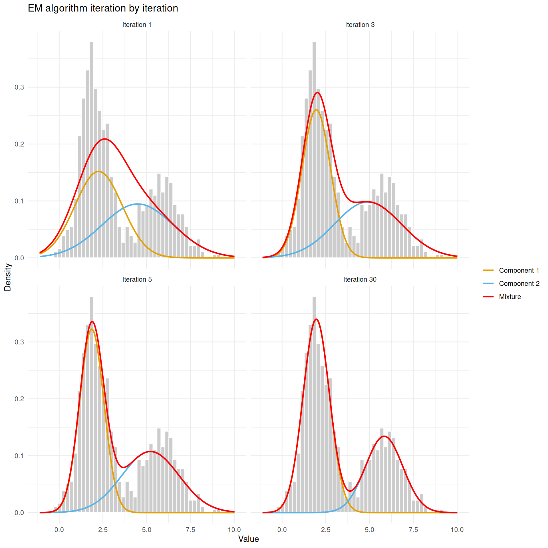

EM at iterations 1, 3, 5, and after convergence. The two Gaussian components (orange and blue curves) gradually separate and fit the data.

Version	Author	Date
ab2ee65	Dave Tang	2026-03-23

At iteration 1, the two components are poorly placed — they are too close together and too wide. By iteration 3, they have started to separate. By convergence, each component sits neatly over one of the two humps and the combined mixture (red) traces the overall shape of the data.

How Responsibilities Evolve

The E-step assigns each data point a responsibility (a probability between 0 and 1) for each component. Let’s see how these responsibilities sharpen over iterations.

resp_iters <- c(1, 3, fit$iterations)
resp_iters <- unique(pmin(resp_iters, fit$iterations))

resp_data <- do.call(rbind, lapply(resp_iters, function(i) {
  data.frame(
    x = x,
    resp_2 = fit$snapshots[[i]]$resp[, 2],
    iteration = paste("Iteration", i)
  )
}))

resp_data$iteration <- factor(resp_data$iteration,
                              levels = paste("Iteration", resp_iters))

ggplot(resp_data, aes(x = x, y = resp_2)) +
  geom_point(alpha = 0.4, size = 0.8, colour = "steelblue") +
  geom_hline(yintercept = 0.5, linetype = "dashed", colour = "grey50") +
  facet_wrap(~iteration, ncol = 1) +
  labs(x = "Value", y = "P(Component 2)",
       title = "How responsibilities sharpen over iterations") +
  theme_minimal()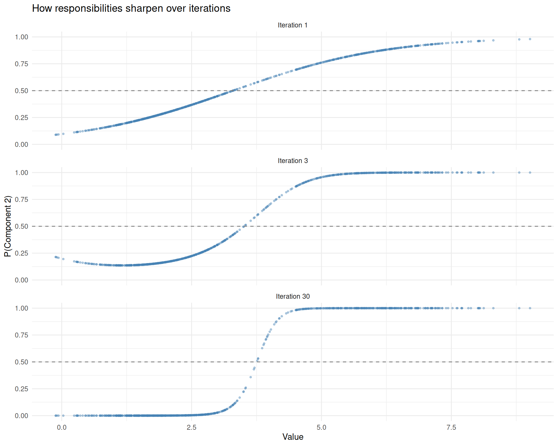

Responsibilities at different iterations. Early on (top), the model is uncertain about most points. By convergence (bottom), assignments are crisp except in the overlap region.

Version	Author	Date
ab2ee65	Dave Tang	2026-03-23

The dashed line at 0.5 marks the decision boundary. Points above the line are assigned to component 2; points below to component 1. In early iterations, many points cluster near 0.5 (the model is uncertain). By convergence, most points are pushed close to 0 or 1, with only the overlap region retaining genuine ambiguity.

Why Does EM Work?

You might wonder: why does this iterative guessing game converge to a good answer instead of going in circles? There is a mathematical guarantee.

The Log-Likelihood Never Decreases

At each iteration, EM is guaranteed to increase (or at least not decrease) the log-likelihood of the data. The log-likelihood measures how well the current parameters explain the observed data. Think of it as a score: higher is better.

# Compute log-likelihood at each iteration
compute_ll <- function(x, mu, sigma, pi_k) {
  K <- length(mu)
  ll <- 0
  for (i in seq_along(x)) {
    p <- 0
    for (k in seq_len(K)) {
      p <- p + pi_k[k] * dnorm(x[i], mu[k], sigma[k])
    }
    ll <- ll + log(p)
  }
  ll
}

ll_values <- sapply(fit$snapshots, function(s) {
  compute_ll(x, s$mu, s$sigma, s$pi_k)
})

df_ll <- data.frame(iteration = seq_along(ll_values), log_likelihood = ll_values)

ggplot(df_ll, aes(x = iteration, y = log_likelihood)) +
  geom_line(linewidth = 1, colour = "darkgreen") +
  geom_point(size = 2, colour = "darkgreen") +
  labs(x = "Iteration", y = "Log-Likelihood",
       title = "Log-likelihood increases at every EM iteration") +
  theme_minimal()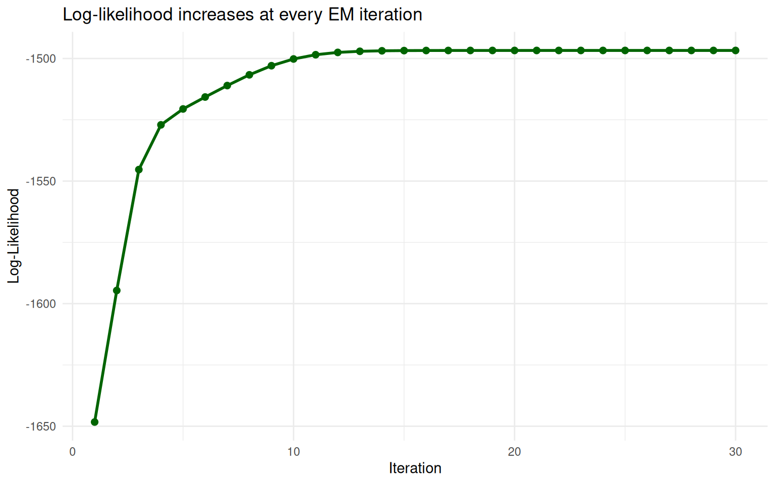

The log-likelihood increases at every EM iteration and plateaus at convergence.

Version	Author	Date
ab2ee65	Dave Tang	2026-03-23

The curve goes up steeply at first (big improvements) then levels off (fine-tuning). EM stops when the improvements become negligibly small.

Local Optima

One important caveat: EM is guaranteed to find a peak in the log-likelihood, but not necessarily the highest peak. The log-likelihood surface can have multiple peaks (local optima), and which one EM finds depends on where it starts.

This means initialisation matters. Let’s demonstrate this by running EM with two different starting points.

# Good initialisation
fit_good <- em_gaussian(x, K = 2)

# Force a bad initialisation by hacking the function
em_gaussian_custom <- function(x, mu_init, sigma_init, pi_init,
                               max_iter = 30, tol = 1e-6) {
  n <- length(x)
  K <- length(mu_init)
  mu <- mu_init
  sigma <- sigma_init
  pi_k <- pi_init

  for (iter in seq_len(max_iter)) {
    resp <- matrix(0, nrow = n, ncol = K)
    for (k in seq_len(K)) {
      resp[, k] <- pi_k[k] * dnorm(x, mean = mu[k], sd = sigma[k])
    }
    resp <- resp / rowSums(resp)

    N_k <- colSums(resp)
    mu_new <- colSums(resp * x) / N_k
    sigma_new <- sqrt(colSums(resp * outer(x, mu_new, "-")^2) / N_k)
    pi_new <- N_k / n

    if (max(abs(mu_new - mu)) < tol) break
    mu <- mu_new
    sigma <- sigma_new
    pi_k <- pi_new
  }
  list(mu = mu_new, sigma = sigma_new, pi_k = pi_new)
}

# Bad initialisation: both means on the same side
fit_bad <- em_gaussian_custom(x,
  mu_init = c(5.5, 6.5),
  sigma_init = c(1, 1),
  pi_init = c(0.5, 0.5)
)

# Plot both results
x_grid <- seq(min(x) - 1, max(x) + 1, length.out = 500)

df_good <- data.frame(
  x = x_grid,
  density = fit_good$pi_k[1] * dnorm(x_grid, fit_good$mu[1], fit_good$sigma[1]) +
    fit_good$pi_k[2] * dnorm(x_grid, fit_good$mu[2], fit_good$sigma[2]),
  init = "Good initialisation"
)
df_bad <- data.frame(
  x = x_grid,
  density = fit_bad$pi_k[1] * dnorm(x_grid, fit_bad$mu[1], fit_bad$sigma[1]) +
    fit_bad$pi_k[2] * dnorm(x_grid, fit_bad$mu[2], fit_bad$sigma[2]),
  init = "Bad initialisation"
)

df_inits <- rbind(df_good, df_bad)

ggplot() +
  geom_histogram(data = data.frame(x = x), aes(x = x, y = after_stat(density)),
                 bins = 50, fill = "grey80", colour = "white") +
  geom_line(data = df_inits, aes(x = x, y = density, colour = init),
            linewidth = 1) +
  labs(x = "Value", y = "Density", colour = "",
       title = "The same algorithm, two different starting points") +
  theme_minimal()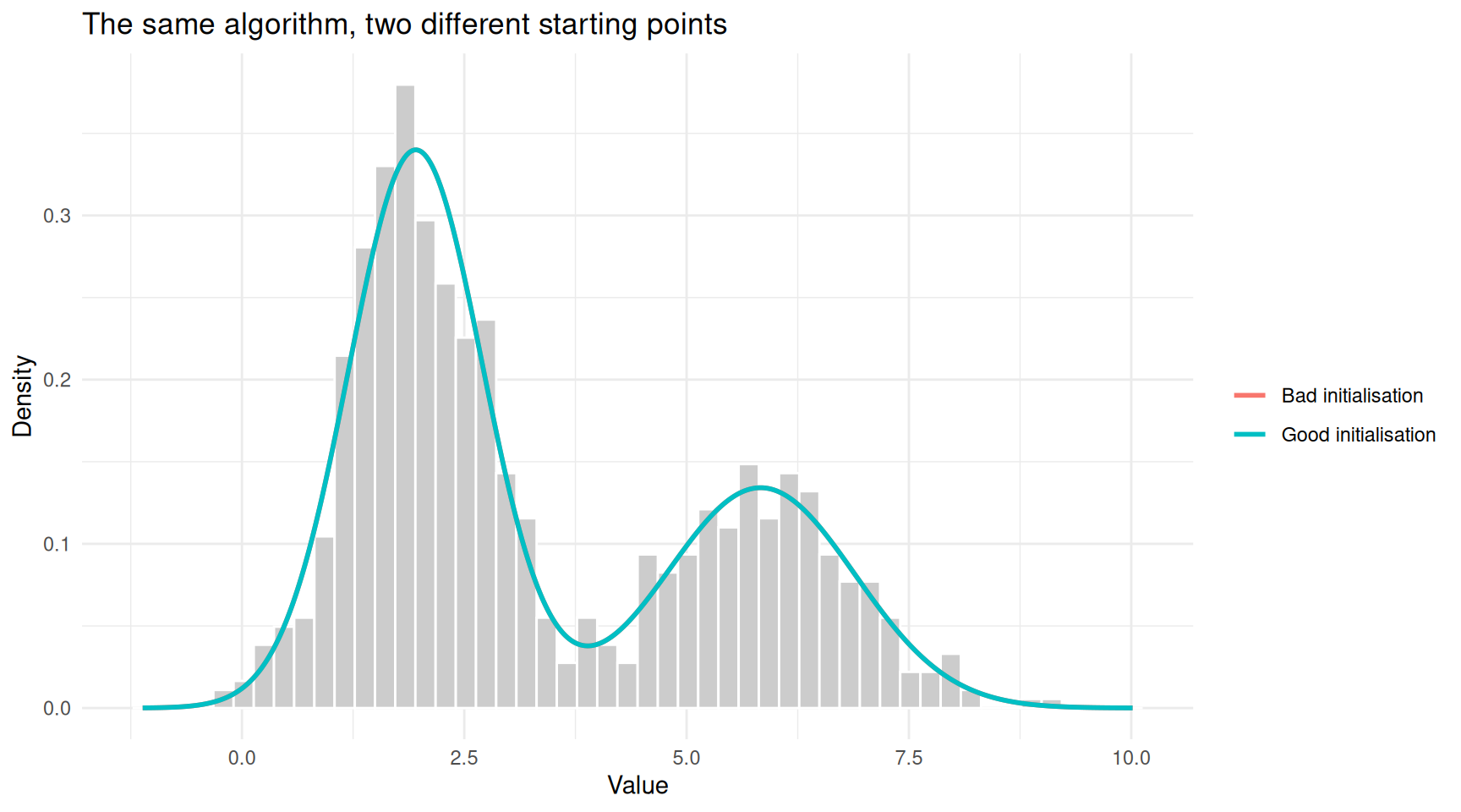

Different starting points can lead to different solutions. Here, a poor initialisation gets stuck.

Version	Author	Date
ab2ee65	Dave Tang	2026-03-23

cat("Good initialisation:\n")

Good initialisation:

cat(sprintf("  Component 1: mean = %.2f, sd = %.2f\n", fit_good$mu[1], fit_good$sigma[1]))

  Component 1: mean = 1.95, sd = 0.76

cat(sprintf("  Component 2: mean = %.2f, sd = %.2f\n\n", fit_good$mu[2], fit_good$sigma[2]))

  Component 2: mean = 5.83, sd = 1.06

cat("Bad initialisation:\n")

Bad initialisation:

cat(sprintf("  Component 1: mean = %.2f, sd = %.2f\n", fit_bad$mu[1], fit_bad$sigma[1]))

  Component 1: mean = 1.95, sd = 0.76

cat(sprintf("  Component 2: mean = %.2f, sd = %.2f\n", fit_bad$mu[2], fit_bad$sigma[2]))

  Component 2: mean = 5.83, sd = 1.06

In practice, the standard defence against local optima is to run EM multiple times with different random starting points and keep the result with the highest log-likelihood. Packages like mclust in R do this automatically.

The General Pattern

EM always follows the same template, regardless of the specific model:

Step	What you do	Two-coin example	Grading example	Gaussian mixture
Hidden data	Identify what is unobserved	Which coin was used in each round	Which TA graded each assignment	Which component generated each data point
Initialise	Make an initial guess for the parameters	\(\theta_A = 0.6\), \(\theta_B = 0.5\)	Mean scores of 75 and 70	Means, SDs, and weights
E-step	Compute the expected value of the hidden data, given current parameters	P(coin A \| round data) for each round	P(Alice \| score) for each assignment	P(component \(k\) \| data point) for each point
M-step	Re-estimate parameters, treating the expected hidden data as if it were real	Weighted proportion of heads for each coin	Weighted mean score for each TA	Weighted mean, SD, and proportion for each component
Repeat	Until parameters stop changing	—	—	—

The beauty of EM is that both the E-step and the M-step are usually easy problems on their own. The E-step is just plugging numbers into a formula. The M-step is often a familiar calculation (like computing a mean). It is only the combination — the fact that you don’t know the hidden data — that makes the original problem hard. EM turns one hard problem into a sequence of easy ones.

Common Pitfalls

Choosing K

EM assumes you already know the number of components \(K\). In the two-coin problem, we knew there were 2 coins. In practice, you may not know \(K\). Common approaches:

BIC (Bayesian Information Criterion): fit models with different values of \(K\) and pick the one with the best BIC, which balances fit against model complexity. This is what mclust does in R.
Domain knowledge: sometimes the number of groups is known from the subject matter (e.g., two sexes, three treatment arms).

Convergence Speed

EM can be slow when components overlap heavily. In such cases, the responsibilities stay uncertain for many iterations, and the parameters update by tiny amounts. This is usually not a problem in practice (modern computers handle thousands of iterations quickly), but it is worth knowing.

Degenerate Solutions

If a Gaussian component collapses onto a single data point (mean equals that point, standard deviation shrinks to zero), the likelihood goes to infinity. This is a degenerate solution. Well-implemented packages guard against this by adding small regularisation terms or using constrained covariance structures.

Summary

Concept	Plain-language meaning
EM algorithm	An iterative method for estimating parameters when there is hidden (unobserved) information
E-step	“Given my current guesses, how should I fill in the blanks?” — compute soft assignments of hidden variables
M-step	“Given the filled-in blanks, what are the best parameter estimates?” — update parameters using standard formulas
Responsibility	The probability that a particular hidden state generated a particular data point
Log-likelihood	A score that measures how well the current parameters explain the data; EM never decreases it
Local optimum	EM finds a peak, but not necessarily the highest peak; run it multiple times with different starting points
Convergence	When the parameter updates become negligibly small, the algorithm stops

The EM algorithm is not magic. It is a disciplined way of handling the chicken-and-egg problem that arises whenever you have incomplete data. Once you see it as “guess the hidden stuff, update your parameters, repeat”, the notation in textbooks becomes much less intimidating.

Session Info

sessionInfo()

R version 4.5.2 (2025-10-31)
Platform: x86_64-pc-linux-gnu
Running under: Ubuntu 24.04.4 LTS

Matrix products: default
BLAS:   /usr/lib/x86_64-linux-gnu/openblas-pthread/libblas.so.3 
LAPACK: /usr/lib/x86_64-linux-gnu/openblas-pthread/libopenblasp-r0.3.26.so;  LAPACK version 3.12.0

locale:
 [1] LC_CTYPE=en_US.UTF-8       LC_NUMERIC=C              
 [3] LC_TIME=en_US.UTF-8        LC_COLLATE=en_US.UTF-8    
 [5] LC_MONETARY=en_US.UTF-8    LC_MESSAGES=en_US.UTF-8   
 [7] LC_PAPER=en_US.UTF-8       LC_NAME=C                 
 [9] LC_ADDRESS=C               LC_TELEPHONE=C            
[11] LC_MEASUREMENT=en_US.UTF-8 LC_IDENTIFICATION=C       

time zone: Etc/UTC
tzcode source: system (glibc)

attached base packages:
[1] stats     graphics  grDevices utils     datasets  methods   base     

other attached packages:
[1] ggplot2_4.0.2   workflowr_1.7.2

loaded via a namespace (and not attached):
 [1] gtable_0.3.6       jsonlite_2.0.0     dplyr_1.2.0        compiler_4.5.2    
 [5] promises_1.5.0     tidyselect_1.2.1   Rcpp_1.1.1         stringr_1.6.0     
 [9] git2r_0.36.2       callr_3.7.6        later_1.4.7        jquerylib_0.1.4   
[13] scales_1.4.0       yaml_2.3.12        fastmap_1.2.0      R6_2.6.1          
[17] labeling_0.4.3     generics_0.1.4     knitr_1.51         tibble_3.3.1      
[21] rprojroot_2.1.1    RColorBrewer_1.1-3 bslib_0.10.0       pillar_1.11.1     
[25] rlang_1.1.7        cachem_1.1.0       stringi_1.8.7      httpuv_1.6.16     
[29] xfun_0.56          S7_0.2.1           getPass_0.2-4      fs_1.6.6          
[33] sass_0.4.10        otel_0.2.0         cli_3.6.5          withr_3.0.2       
[37] magrittr_2.0.4     ps_1.9.1           digest_0.6.39      grid_4.5.2        
[41] processx_3.8.6     rstudioapi_0.18.0  lifecycle_1.0.5    vctrs_0.7.1       
[45] evaluate_1.0.5     glue_1.8.0         farver_2.1.2       whisker_0.4.1     
[49] rmarkdown_2.30     httr_1.4.8         tools_4.5.2        pkgconfig_2.0.3   
[53] htmltools_0.5.9

sessionInfo()

R version 4.5.2 (2025-10-31)
Platform: x86_64-pc-linux-gnu
Running under: Ubuntu 24.04.4 LTS

Matrix products: default
BLAS:   /usr/lib/x86_64-linux-gnu/openblas-pthread/libblas.so.3 
LAPACK: /usr/lib/x86_64-linux-gnu/openblas-pthread/libopenblasp-r0.3.26.so;  LAPACK version 3.12.0

locale:
 [1] LC_CTYPE=en_US.UTF-8       LC_NUMERIC=C              
 [3] LC_TIME=en_US.UTF-8        LC_COLLATE=en_US.UTF-8    
 [5] LC_MONETARY=en_US.UTF-8    LC_MESSAGES=en_US.UTF-8   
 [7] LC_PAPER=en_US.UTF-8       LC_NAME=C                 
 [9] LC_ADDRESS=C               LC_TELEPHONE=C            
[11] LC_MEASUREMENT=en_US.UTF-8 LC_IDENTIFICATION=C       

time zone: Etc/UTC
tzcode source: system (glibc)

attached base packages:
[1] stats     graphics  grDevices utils     datasets  methods   base     

other attached packages:
[1] ggplot2_4.0.2   workflowr_1.7.2

loaded via a namespace (and not attached):
 [1] gtable_0.3.6       jsonlite_2.0.0     dplyr_1.2.0        compiler_4.5.2    
 [5] promises_1.5.0     tidyselect_1.2.1   Rcpp_1.1.1         stringr_1.6.0     
 [9] git2r_0.36.2       callr_3.7.6        later_1.4.7        jquerylib_0.1.4   
[13] scales_1.4.0       yaml_2.3.12        fastmap_1.2.0      R6_2.6.1          
[17] labeling_0.4.3     generics_0.1.4     knitr_1.51         tibble_3.3.1      
[21] rprojroot_2.1.1    RColorBrewer_1.1-3 bslib_0.10.0       pillar_1.11.1     
[25] rlang_1.1.7        cachem_1.1.0       stringi_1.8.7      httpuv_1.6.16     
[29] xfun_0.56          S7_0.2.1           getPass_0.2-4      fs_1.6.6          
[33] sass_0.4.10        otel_0.2.0         cli_3.6.5          withr_3.0.2       
[37] magrittr_2.0.4     ps_1.9.1           digest_0.6.39      grid_4.5.2        
[41] processx_3.8.6     rstudioapi_0.18.0  lifecycle_1.0.5    vctrs_0.7.1       
[45] evaluate_1.0.5     glue_1.8.0         farver_2.1.2       whisker_0.4.1     
[49] rmarkdown_2.30     httr_1.4.8         tools_4.5.2        pkgconfig_2.0.3   
[53] htmltools_0.5.9

The Expectation-Maximisation (EM) Algorithm

2026-03-24