Last updated: 2026-02-04

Checks: 7 0

Knit directory: muse/

This reproducible R Markdown analysis was created with workflowr (version 1.7.1). The Checks tab describes the reproducibility checks that were applied when the results were created. The Past versions tab lists the development history.

R Markdown file: up-to-date

Great! Since the R Markdown file has been committed to the Git repository, you know the exact version of the code that produced these results.

Environment: empty

Great job! The global environment was empty. Objects defined in the global environment can affect the analysis in your R Markdown file in unknown ways. For reproduciblity it’s best to always run the code in an empty environment.

Seed: set.seed(20200712)

The command set.seed(20200712) was run prior to running the code in the R Markdown file. Setting a seed ensures that any results that rely on randomness, e.g. subsampling or permutations, are reproducible.

Session information: recorded

Great job! Recording the operating system, R version, and package versions is critical for reproducibility.

Cache: none

Nice! There were no cached chunks for this analysis, so you can be confident that you successfully produced the results during this run.

File paths: relative

Great job! Using relative paths to the files within your workflowr project makes it easier to run your code on other machines.

Repository version: 2a88aef

Great! You are using Git for version control. Tracking code development and connecting the code version to the results is critical for reproducibility.

The results in this page were generated with repository version 2a88aef. See the Past versions tab to see a history of the changes made to the R Markdown and HTML files.

Note that you need to be careful to ensure that all relevant files for the analysis have been committed to Git prior to generating the results (you can use wflow_publish or wflow_git_commit). workflowr only checks the R Markdown file, but you know if there are other scripts or data files that it depends on. Below is the status of the Git repository when the results were generated:


Ignored files:
    Ignored:    .Rproj.user/
    Ignored:    data/1M_neurons_filtered_gene_bc_matrices_h5.h5
    Ignored:    data/293t/
    Ignored:    data/293t_3t3_filtered_gene_bc_matrices.tar.gz
    Ignored:    data/293t_filtered_gene_bc_matrices.tar.gz
    Ignored:    data/5k_Human_Donor1_PBMC_3p_gem-x_5k_Human_Donor1_PBMC_3p_gem-x_count_sample_filtered_feature_bc_matrix.h5
    Ignored:    data/5k_Human_Donor2_PBMC_3p_gem-x_5k_Human_Donor2_PBMC_3p_gem-x_count_sample_filtered_feature_bc_matrix.h5
    Ignored:    data/5k_Human_Donor3_PBMC_3p_gem-x_5k_Human_Donor3_PBMC_3p_gem-x_count_sample_filtered_feature_bc_matrix.h5
    Ignored:    data/5k_Human_Donor4_PBMC_3p_gem-x_5k_Human_Donor4_PBMC_3p_gem-x_count_sample_filtered_feature_bc_matrix.h5
    Ignored:    data/97516b79-8d08-46a6-b329-5d0a25b0be98.h5ad
    Ignored:    data/Parent_SC3v3_Human_Glioblastoma_filtered_feature_bc_matrix.tar.gz
    Ignored:    data/brain_counts/
    Ignored:    data/cl.obo
    Ignored:    data/cl.owl
    Ignored:    data/jurkat/
    Ignored:    data/jurkat:293t_50:50_filtered_gene_bc_matrices.tar.gz
    Ignored:    data/jurkat_293t/
    Ignored:    data/jurkat_filtered_gene_bc_matrices.tar.gz
    Ignored:    data/pbmc20k/
    Ignored:    data/pbmc20k_seurat/
    Ignored:    data/pbmc3k.csv
    Ignored:    data/pbmc3k.csv.gz
    Ignored:    data/pbmc3k.h5ad
    Ignored:    data/pbmc3k/
    Ignored:    data/pbmc3k_bpcells_mat/
    Ignored:    data/pbmc3k_export.mtx
    Ignored:    data/pbmc3k_matrix.mtx
    Ignored:    data/pbmc3k_seurat.rds
    Ignored:    data/pbmc4k_filtered_gene_bc_matrices.tar.gz
    Ignored:    data/pbmc_1k_v3_filtered_feature_bc_matrix.h5
    Ignored:    data/pbmc_1k_v3_raw_feature_bc_matrix.h5
    Ignored:    data/refdata-gex-GRCh38-2020-A.tar.gz
    Ignored:    data/seurat_1m_neuron.rds
    Ignored:    data/t_3k_filtered_gene_bc_matrices.tar.gz
    Ignored:    r_packages_4.4.1/
    Ignored:    r_packages_4.5.0/

Untracked files:
    Untracked:  .claude/
    Untracked:  CLAUDE.md
    Untracked:  analysis/bioc.Rmd
    Untracked:  analysis/bioc_scrnaseq.Rmd
    Untracked:  analysis/chick_weight.Rmd
    Untracked:  analysis/likelihood.Rmd
    Untracked:  bpcells_matrix/
    Untracked:  data/Caenorhabditis_elegans.WBcel235.113.gtf.gz
    Untracked:  data/GCF_043380555.1-RS_2024_12_gene_ontology.gaf.gz
    Untracked:  data/SeuratObj.rds
    Untracked:  data/arab.rds
    Untracked:  data/astronomicalunit.csv
    Untracked:  data/femaleMiceWeights.csv
    Untracked:  data/lung_bcell.rds
    Untracked:  m3/
    Untracked:  women.json

Unstaged changes:
    Modified:   analysis/isoform_switch_analyzer.Rmd
    Modified:   analysis/linear_models.Rmd

Note that any generated files, e.g. HTML, png, CSS, etc., are not included in this status report because it is ok for generated content to have uncommitted changes.

These are the previous versions of the repository in which changes were made to the R Markdown (analysis/fitting.Rmd) and HTML (docs/fitting.html) files. If you’ve configured a remote Git repository (see ?wflow_git_remote), click on the hyperlinks in the table below to view the files as they were in that past version.

File	Version	Author	Date	Message
Rmd	2a88aef	Dave Tang	2026-02-04	Add explanations on fitting
html	b2fed23	Dave Tang	2025-09-02	Build site.
Rmd	15473ba	Dave Tang	2025-09-02	Negative binomial
html	161c3d6	Dave Tang	2025-09-02	Build site.
Rmd	3160792	Dave Tang	2025-09-02	Gamma distribution
html	779b385	Dave Tang	2025-09-02	Build site.
Rmd	5a74914	Dave Tang	2025-09-02	Fitting a distribution

Introduction

When we say a “distribution was fit to” data, it means we assume the data comes from some probability distribution and we estimate the distribution’s parameters so the model best represents the observed values.

Why Fit Distributions?

Distribution fitting is useful for:

Understanding data: Identifying the underlying process that generated your data
Simulation: Generating synthetic data with similar properties
Prediction: Calculating probabilities of future events
Statistical testing: Many tests assume specific distributions
Quality control: Monitoring processes in manufacturing and other fields

Maximum Likelihood Estimation

The most common method for fitting distributions is Maximum Likelihood Estimation (MLE). The idea is to find parameter values that make the observed data most probable.

For example, if we have data and assume it comes from a normal distribution, MLE finds the mean (\(\mu\)) and standard deviation (\(\sigma\)) that maximise the likelihood of observing that data.

The likelihood function for n independent observations is:

\[L(\theta | x_1, ..., x_n) = \prod_{i=1}^{n} f(x_i | \theta)\]

where \(f\) is the probability density function and \(\theta\) represents the parameters. In practice, we maximise the log-likelihood for computational convenience.

Fitting Distributions with MASS

The MASS::fitdistr() function fits univariate distributions using maximum likelihood estimation. Let’s work through several examples.

Example 1: Normal Distribution

The normal (Gaussian) distribution is characterised by two parameters: mean (\(\mu\)) and standard deviation (\(\sigma\)).

set.seed(1984)
eg1 <- rnorm(100, mean = 5, sd = 2)

Fit a normal distribution to the data:

eg1_fit <- fitdistr(eg1, "normal")
eg1_fit

     mean        sd   
  5.062545   1.873380 
 (0.187338) (0.132468)

Understanding the Output

The output shows:

Estimated parameters: mean = 5.063, sd = 1.873
Standard errors: The values in parentheses indicate uncertainty in the estimates

The true parameters were mean = 5 and sd = 2. Our estimates are close, demonstrating that MLE recovers the true parameters reasonably well with 100 observations.

Visualising the Fit

It’s important to visually verify that the fitted distribution matches the data:

ggplot(data.frame(x = eg1), aes(x)) +
  geom_histogram(aes(y = after_stat(density)), bins = 20,
                 fill = "steelblue", colour = "white", alpha = 0.7) +
  stat_function(fun = dnorm,
                args = list(mean = eg1_fit$estimate['mean'],
                            sd = eg1_fit$estimate['sd']),
                colour = "red", linewidth = 1) +
  labs(title = "Normal Distribution Fit",
       subtitle = paste0("Estimated: mean = ", round(eg1_fit$estimate['mean'], 2),
                        ", sd = ", round(eg1_fit$estimate['sd'], 2)),
       x = "Value", y = "Density") +
  theme_minimal()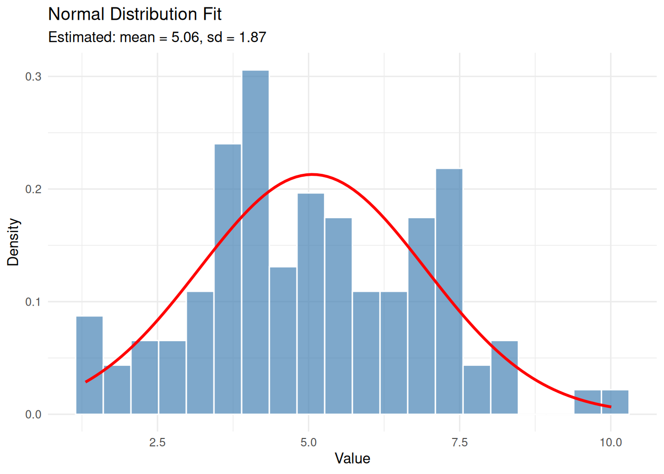

The red curve shows the fitted normal distribution overlaid on the histogram of our data.

Example 2: Poisson Distribution

The Poisson distribution models count data and has a single parameter \(\lambda\) (lambda), which represents both the mean and variance.

set.seed(1984)
eg2 <- rpois(100, lambda = 3)
eg2_fit <- fitdistr(eg2, "Poisson")
eg2_fit

    lambda  
  3.1000000 
 (0.1760682)

The estimated \(\lambda\) = 3.1 is close to the true value of 3.

# Create comparison data
x_vals <- 0:max(eg2)
observed <- table(factor(eg2, levels = x_vals)) / length(eg2)
expected <- dpois(x_vals, lambda = eg2_fit$estimate['lambda'])

plot_data <- data.frame(
  x = rep(x_vals, 2),
  probability = c(as.numeric(observed), expected),
  type = rep(c("Observed", "Fitted"), each = length(x_vals))
)

ggplot(plot_data, aes(x, probability, fill = type)) +
  geom_bar(stat = "identity", position = "dodge", alpha = 0.7) +
  scale_fill_manual(values = c("Observed" = "steelblue", "Fitted" = "red")) +
  labs(title = "Poisson Distribution Fit",
       subtitle = paste0("Estimated: lambda = ", round(eg2_fit$estimate['lambda'], 2)),
       x = "Count", y = "Probability", fill = "") +
  theme_minimal()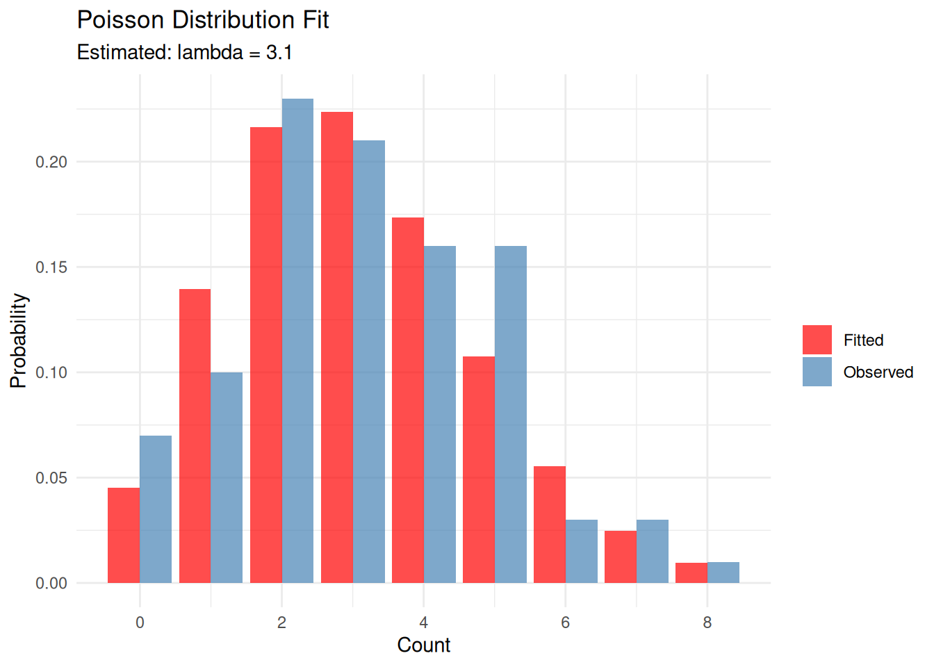

Example 3: Gamma Distribution

The gamma distribution is useful for modelling positive continuous data, such as waiting times or rainfall amounts. It has two parameters: shape (\(\alpha\)) and rate (\(\beta\)).

set.seed(1984)
eg3 <- rgamma(300, shape = 2, rate = 3)

eg3_fit <- fitdistr(eg3, "gamma")

Warning in densfun(x, parm[1], parm[2], ...): NaNs produced

eg3_fit

     shape       rate   
  2.0425966   3.1910159 
 (0.1550892) (0.2744437)

True parameters: shape = 2, rate = 3. The estimates are reasonably close.

ggplot(data.frame(x = eg3), aes(x)) +
  geom_histogram(aes(y = after_stat(density)), bins = 30,
                 fill = "steelblue", colour = "white", alpha = 0.7) +
  stat_function(fun = dgamma,
                args = list(shape = eg3_fit$estimate['shape'],
                            rate = eg3_fit$estimate['rate']),
                colour = "red", linewidth = 1) +
  labs(title = "Gamma Distribution Fit",
       subtitle = paste0("Estimated: shape = ", round(eg3_fit$estimate['shape'], 2),
                        ", rate = ", round(eg3_fit$estimate['rate'], 2)),
       x = "Value", y = "Density") +
  theme_minimal()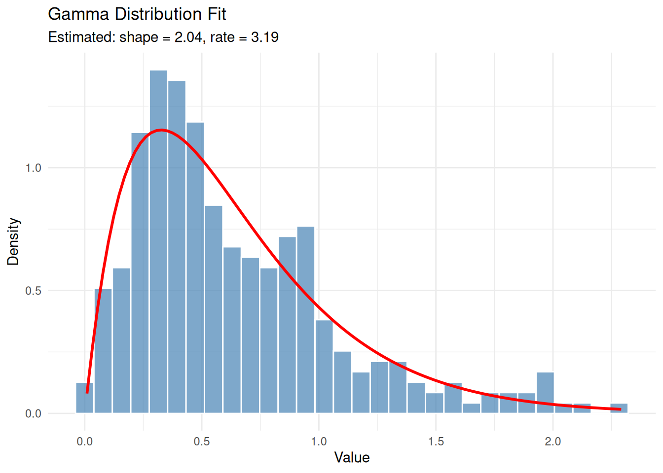

Example 4: Negative Binomial Distribution

The negative binomial distribution is useful for overdispersed count data (when variance exceeds the mean). It has two parameters: size (\(r\)) and mu (\(\mu\)).

set.seed(1984)
eg4 <- rnbinom(100, mu = 10, size = 5)

eg4_fit <- fitdistr(eg4, "negative binomial")
eg4_fit

     size         mu    
  4.9764745   9.7999979 
 (1.0492499) (0.5394329)

x_vals <- 0:max(eg4)
observed <- table(factor(eg4, levels = x_vals)) / length(eg4)
expected <- dnbinom(x_vals, mu = eg4_fit$estimate['mu'], size = eg4_fit$estimate['size'])

plot_data <- data.frame(
  x = rep(x_vals, 2),
  probability = c(as.numeric(observed), expected),
  type = rep(c("Observed", "Fitted"), each = length(x_vals))
)

ggplot(plot_data, aes(x, probability, fill = type)) +
  geom_bar(stat = "identity", position = "dodge", alpha = 0.7) +
  scale_fill_manual(values = c("Observed" = "steelblue", "Fitted" = "red")) +
  labs(title = "Negative Binomial Distribution Fit",
       subtitle = paste0("Estimated: size = ", round(eg4_fit$estimate['size'], 2),
                        ", mu = ", round(eg4_fit$estimate['mu'], 2)),
       x = "Count", y = "Probability", fill = "") +
  theme_minimal()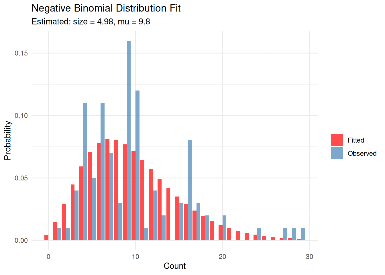

Supported Distributions

MASS::fitdistr() supports the following distributions:

“beta”
“cauchy”
“chi-squared”
“exponential”
“gamma”
“geometric”
“log-normal”
“lognormal”
“logistic”
“negative binomial”
“normal”
“Poisson”
“t”
“weibull”

Comparing Model Fits

When multiple distributions could plausibly fit your data, you need methods to compare them.

Akaike Information Criterion (AIC)

The Akaike Information Criterion (AIC) measures how well a model fits the data while penalising model complexity:

\[AIC = 2k - 2\ln(L)\]

where \(k\) is the number of parameters and \(L\) is the maximum likelihood. Lower AIC values indicate better fit. The penalty term (2k) prevents overfitting by discouraging unnecessarily complex models.

Example: Normal vs Exponential

Let’s compare normal and exponential fits for our normally distributed data:

set.seed(1984)
eg1 <- rnorm(100, mean = 5, sd = 2)

eg1_norm <- fitdistr(eg1, "normal")
eg1_exp <- fitdistr(eg1, "exponential")

AIC(eg1_norm, eg1_exp)

         df      AIC
eg1_norm  2 413.3365
eg1_exp   1 526.3739

The normal distribution has a much lower AIC, correctly indicating it’s a better fit. We can also visualise why:

ggplot(data.frame(x = eg1), aes(x)) +
  geom_histogram(aes(y = after_stat(density)), bins = 20,
                 fill = "grey70", colour = "white") +
  stat_function(fun = dnorm,
                args = list(mean = eg1_norm$estimate['mean'],
                            sd = eg1_norm$estimate['sd']),
                aes(colour = "Normal"), linewidth = 1) +
  stat_function(fun = dexp,
                args = list(rate = eg1_exp$estimate['rate']),
                aes(colour = "Exponential"), linewidth = 1) +
  scale_colour_manual(values = c("Normal" = "blue", "Exponential" = "red")) +
  labs(title = "Comparing Normal vs Exponential Fit",
       x = "Value", y = "Density", colour = "Distribution") +
  theme_minimal()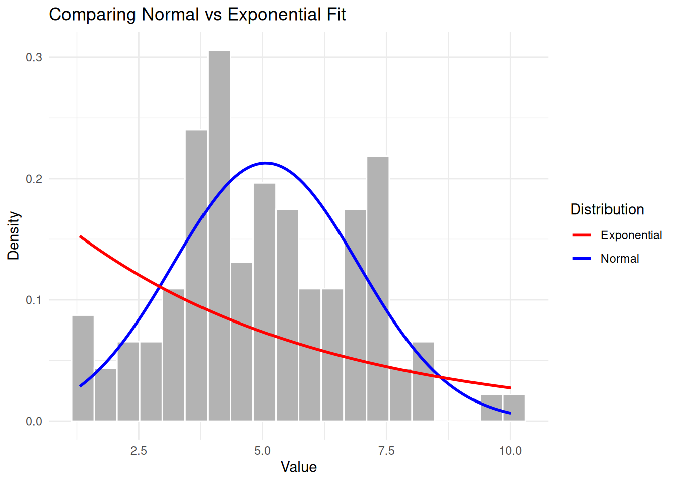

The exponential distribution clearly doesn’t capture the symmetric, bell-shaped nature of the data.

Bayesian Information Criterion (BIC)

BIC is similar to AIC but applies a stronger penalty for model complexity:

\[BIC = k\ln(n) - 2\ln(L)\]

where \(n\) is the sample size. BIC tends to favour simpler models than AIC.

BIC(eg1_norm, eg1_exp)

         df      BIC
eg1_norm  2 418.5469
eg1_exp   1 528.9791

Both criteria agree that the normal distribution is the better fit.

Example: Choosing Between Related Distributions

Sometimes the choice is less obvious. Consider count data that might follow either a Poisson or negative binomial distribution:

set.seed(1984)
# Generate overdispersed count data
overdispersed <- rnbinom(200, mu = 5, size = 2)

# Fit both distributions
pois_fit <- fitdistr(overdispersed, "Poisson")
nb_fit <- fitdistr(overdispersed, "negative binomial")

# Compare AIC
AIC(pois_fit, nb_fit)

         df      AIC
pois_fit  1 1371.432
nb_fit    2 1081.379

x_vals <- 0:max(overdispersed)
observed <- table(factor(overdispersed, levels = x_vals)) / length(overdispersed)
pois_expected <- dpois(x_vals, lambda = pois_fit$estimate['lambda'])
nb_expected <- dnbinom(x_vals, mu = nb_fit$estimate['mu'], size = nb_fit$estimate['size'])

plot_data <- data.frame(
  x = rep(x_vals, 3),
  probability = c(as.numeric(observed), pois_expected, nb_expected),
  type = rep(c("Observed", "Poisson", "Negative Binomial"), each = length(x_vals))
)

ggplot(plot_data, aes(x, probability, fill = type)) +
  geom_bar(stat = "identity", position = "dodge", alpha = 0.7) +
  scale_fill_manual(values = c("Observed" = "grey50",
                               "Poisson" = "steelblue",
                               "Negative Binomial" = "darkred")) +
  labs(title = "Poisson vs Negative Binomial Fit",
       subtitle = "For overdispersed count data",
       x = "Count", y = "Probability", fill = "") +
  theme_minimal()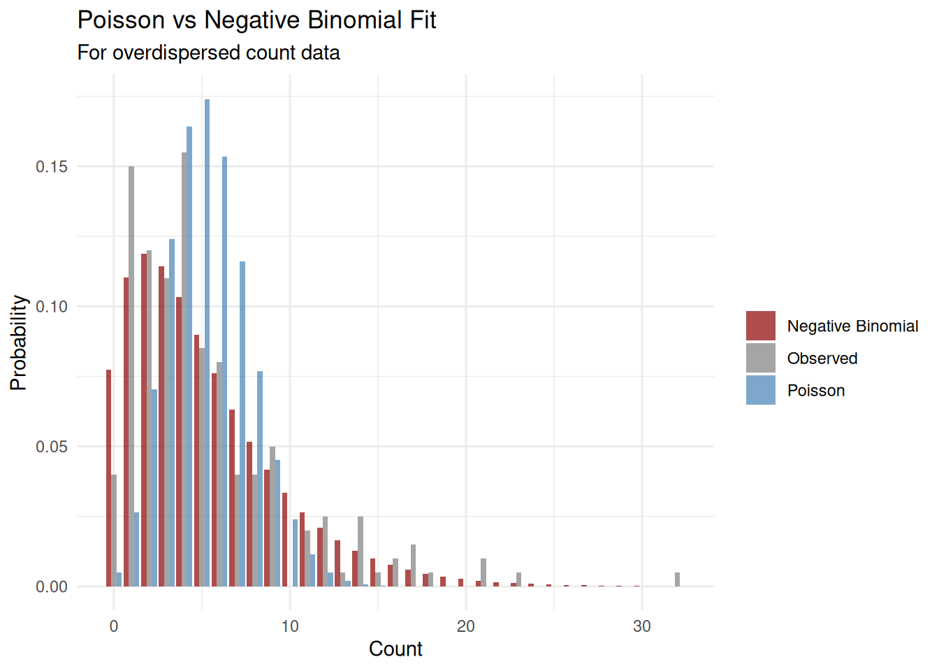

The negative binomial has lower AIC because it can accommodate the overdispersion (variance > mean) in the data, which the Poisson cannot.

Assessing Goodness of Fit

Beyond comparing models, you should assess whether any distribution fits well in absolute terms.

Q-Q Plots

Quantile-Quantile (Q-Q) plots compare the quantiles of your data against theoretical quantiles. If the data follows the assumed distribution, points should fall along the diagonal line.

# Q-Q plot for normal fit
eg1_sorted <- sort(eg1)
theoretical_quantiles <- qnorm(ppoints(length(eg1)),
                               mean = eg1_fit$estimate['mean'],
                               sd = eg1_fit$estimate['sd'])

ggplot(data.frame(theoretical = theoretical_quantiles, observed = eg1_sorted),
       aes(theoretical, observed)) +
  geom_point(alpha = 0.6) +
  geom_abline(slope = 1, intercept = 0, colour = "red", linetype = "dashed") +
  labs(title = "Q-Q Plot: Normal Distribution",
       x = "Theoretical Quantiles", y = "Observed Quantiles") +
  theme_minimal()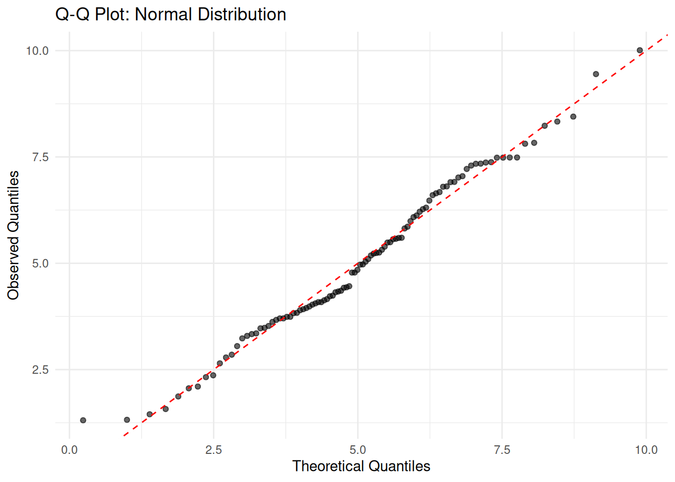

Points closely following the diagonal line indicate a good fit.

Kolmogorov-Smirnov Test

The Kolmogorov-Smirnov test formally tests whether data comes from a specified distribution:

ks.test(eg1, "pnorm",
        mean = eg1_fit$estimate['mean'],
        sd = eg1_fit$estimate['sd'])


    Asymptotic one-sample Kolmogorov-Smirnov test

data:  eg1
D = 0.086058, p-value = 0.4494
alternative hypothesis: two-sided

A large p-value (> 0.05) suggests we cannot reject the hypothesis that the data comes from the fitted distribution.

Practical Considerations

Sample Size

Larger samples produce more reliable parameter estimates:

set.seed(1984)
true_mean <- 10
true_sd <- 3

# Compare estimates at different sample sizes
sample_sizes <- c(20, 50, 100, 500, 1000)
results <- lapply(sample_sizes, function(n) {
  x <- rnorm(n, mean = true_mean, sd = true_sd)
  fit <- fitdistr(x, "normal")
  data.frame(
    n = n,
    est_mean = fit$estimate['mean'],
    est_sd = fit$estimate['sd'],
    se_mean = fit$sd['mean'],
    se_sd = fit$sd['sd']
  )
})

results_df <- do.call(rbind, results)
results_df

         n  est_mean   est_sd    se_mean      se_sd
mean    20 10.382167 3.026534 0.67675348 0.47853697
mean1   50 10.226157 2.746529 0.38841779 0.27465285
mean2  100  9.604006 2.743902 0.27439024 0.19402320
mean3  500  9.804773 3.020142 0.13506485 0.09550527
mean4 1000  9.954271 3.011147 0.09522084 0.06733130

Notice how standard errors decrease as sample size increases.

Starting Values

For some distributions, fitdistr() may need starting values to converge:

set.seed(1984)
weibull_data <- rweibull(100, shape = 2, scale = 5)

# Provide starting values for Weibull
weibull_fit <- fitdistr(weibull_data, "weibull",
                        start = list(shape = 1, scale = 1))

Warning in densfun(x, parm[1], parm[2], ...): NaNs produced
Warning in densfun(x, parm[1], parm[2], ...): NaNs produced
Warning in densfun(x, parm[1], parm[2], ...): NaNs produced
Warning in densfun(x, parm[1], parm[2], ...): NaNs produced

weibull_fit

     shape       scale  
  1.8967375   4.8896060 
 (0.1458478) (0.2720805)

Accessing Fit Components

The fitted object contains useful information:

# Parameter estimates
eg1_fit$estimate

    mean       sd 
5.062545 1.873380

# Standard errors
eg1_fit$sd

    mean       sd 
0.187338 0.132468

# Log-likelihood
eg1_fit$loglik

[1] -204.6683

# Variance-covariance matrix
eg1_fit$vcov

           mean         sd
mean 0.03509552 0.00000000
sd   0.00000000 0.01754776

Summary

Key points for distribution fitting:

Maximum Likelihood Estimation finds parameters that make observed data most probable
Always visualise the fitted distribution against your data
Compare models using AIC or BIC (lower is better)
Assess goodness of fit with Q-Q plots or formal tests
Larger samples give more reliable estimates
Consider the theoretical basis for choosing a distribution, not just statistical fit

sessionInfo()

R version 4.5.0 (2025-04-11)
Platform: x86_64-pc-linux-gnu
Running under: Ubuntu 24.04.3 LTS

Matrix products: default
BLAS:   /usr/lib/x86_64-linux-gnu/openblas-pthread/libblas.so.3 
LAPACK: /usr/lib/x86_64-linux-gnu/openblas-pthread/libopenblasp-r0.3.26.so;  LAPACK version 3.12.0

locale:
 [1] LC_CTYPE=en_US.UTF-8       LC_NUMERIC=C              
 [3] LC_TIME=en_US.UTF-8        LC_COLLATE=en_US.UTF-8    
 [5] LC_MONETARY=en_US.UTF-8    LC_MESSAGES=en_US.UTF-8   
 [7] LC_PAPER=en_US.UTF-8       LC_NAME=C                 
 [9] LC_ADDRESS=C               LC_TELEPHONE=C            
[11] LC_MEASUREMENT=en_US.UTF-8 LC_IDENTIFICATION=C       

time zone: Etc/UTC
tzcode source: system (glibc)

attached base packages:
[1] stats     graphics  grDevices utils     datasets  methods   base     

other attached packages:
[1] ggplot2_3.5.2   MASS_7.3-65     workflowr_1.7.1

loaded via a namespace (and not attached):
 [1] gtable_0.3.6       jsonlite_2.0.0     dplyr_1.1.4        compiler_4.5.0    
 [5] promises_1.3.3     tidyselect_1.2.1   Rcpp_1.0.14        stringr_1.5.1     
 [9] git2r_0.36.2       callr_3.7.6        later_1.4.2        jquerylib_0.1.4   
[13] scales_1.4.0       yaml_2.3.10        fastmap_1.2.0      R6_2.6.1          
[17] labeling_0.4.3     generics_0.1.4     knitr_1.50         tibble_3.3.0      
[21] rprojroot_2.0.4    RColorBrewer_1.1-3 bslib_0.9.0        pillar_1.10.2     
[25] rlang_1.1.6        cachem_1.1.0       stringi_1.8.7      httpuv_1.6.16     
[29] xfun_0.52          getPass_0.2-4      fs_1.6.6           sass_0.4.10       
[33] cli_3.6.5          withr_3.0.2        magrittr_2.0.3     ps_1.9.1          
[37] digest_0.6.37      grid_4.5.0         processx_3.8.6     rstudioapi_0.17.1 
[41] lifecycle_1.0.4    vctrs_0.6.5        evaluate_1.0.3     glue_1.8.0        
[45] farver_2.1.2       whisker_0.4.1      rmarkdown_2.29     httr_1.4.7        
[49] tools_4.5.0        pkgconfig_2.0.3    htmltools_0.5.8.1