Understanding R’s Formula Syntax
2025-12-30
Last updated: 2025-12-30
Checks: 7 0
Knit directory: muse/
This reproducible R Markdown analysis was created with workflowr (version 1.7.1). The Checks tab describes the reproducibility checks that were applied when the results were created. The Past versions tab lists the development history.
Great! Since the R Markdown file has been committed to the Git repository, you know the exact version of the code that produced these results.
Great job! The global environment was empty. Objects defined in the global environment can affect the analysis in your R Markdown file in unknown ways. For reproduciblity it’s best to always run the code in an empty environment.
The command set.seed(20200712) was run prior to running
the code in the R Markdown file. Setting a seed ensures that any results
that rely on randomness, e.g. subsampling or permutations, are
reproducible.
Great job! Recording the operating system, R version, and package versions is critical for reproducibility.
Nice! There were no cached chunks for this analysis, so you can be confident that you successfully produced the results during this run.
Great job! Using relative paths to the files within your workflowr project makes it easier to run your code on other machines.
Great! You are using Git for version control. Tracking code development and connecting the code version to the results is critical for reproducibility.
The results in this page were generated with repository version bc7a77d. See the Past versions tab to see a history of the changes made to the R Markdown and HTML files.
Note that you need to be careful to ensure that all relevant files for
the analysis have been committed to Git prior to generating the results
(you can use wflow_publish or
wflow_git_commit). workflowr only checks the R Markdown
file, but you know if there are other scripts or data files that it
depends on. Below is the status of the Git repository when the results
were generated:
Ignored files:
    Ignored:    .Rproj.user/
    Ignored:    data/1M_neurons_filtered_gene_bc_matrices_h5.h5
    Ignored:    data/293t/
    Ignored:    data/293t_3t3_filtered_gene_bc_matrices.tar.gz
    Ignored:    data/293t_filtered_gene_bc_matrices.tar.gz
    Ignored:    data/5k_Human_Donor1_PBMC_3p_gem-x_5k_Human_Donor1_PBMC_3p_gem-x_count_sample_filtered_feature_bc_matrix.h5
    Ignored:    data/5k_Human_Donor2_PBMC_3p_gem-x_5k_Human_Donor2_PBMC_3p_gem-x_count_sample_filtered_feature_bc_matrix.h5
    Ignored:    data/5k_Human_Donor3_PBMC_3p_gem-x_5k_Human_Donor3_PBMC_3p_gem-x_count_sample_filtered_feature_bc_matrix.h5
    Ignored:    data/5k_Human_Donor4_PBMC_3p_gem-x_5k_Human_Donor4_PBMC_3p_gem-x_count_sample_filtered_feature_bc_matrix.h5
    Ignored:    data/97516b79-8d08-46a6-b329-5d0a25b0be98.h5ad
    Ignored:    data/Parent_SC3v3_Human_Glioblastoma_filtered_feature_bc_matrix.tar.gz
    Ignored:    data/brain_counts/
    Ignored:    data/cl.obo
    Ignored:    data/cl.owl
    Ignored:    data/jurkat/
    Ignored:    data/jurkat:293t_50:50_filtered_gene_bc_matrices.tar.gz
    Ignored:    data/jurkat_293t/
    Ignored:    data/jurkat_filtered_gene_bc_matrices.tar.gz
    Ignored:    data/pbmc20k/
    Ignored:    data/pbmc20k_seurat/
    Ignored:    data/pbmc3k.h5ad
    Ignored:    data/pbmc3k/
    Ignored:    data/pbmc3k_bpcells_mat/
    Ignored:    data/pbmc3k_export.mtx
    Ignored:    data/pbmc3k_matrix.mtx
    Ignored:    data/pbmc3k_seurat.rds
    Ignored:    data/pbmc4k_filtered_gene_bc_matrices.tar.gz
    Ignored:    data/pbmc_1k_v3_filtered_feature_bc_matrix.h5
    Ignored:    data/pbmc_1k_v3_raw_feature_bc_matrix.h5
    Ignored:    data/refdata-gex-GRCh38-2020-A.tar.gz
    Ignored:    data/seurat_1m_neuron.rds
    Ignored:    data/t_3k_filtered_gene_bc_matrices.tar.gz
    Ignored:    r_packages_4.4.1/
    Ignored:    r_packages_4.5.0/

Untracked files:
    Untracked:  analysis/bioc.Rmd
    Untracked:  analysis/bioc_scrnaseq.Rmd
    Untracked:  analysis/likelihood.Rmd
    Untracked:  bpcells_matrix/
    Untracked:  data/Caenorhabditis_elegans.WBcel235.113.gtf.gz
    Untracked:  data/GCF_043380555.1-RS_2024_12_gene_ontology.gaf.gz
    Untracked:  data/arab.rds
    Untracked:  data/astronomicalunit.csv
    Untracked:  data/femaleMiceWeights.csv
    Untracked:  data/lung_bcell.rds
    Untracked:  m3/
    Untracked:  women.json

Unstaged changes:
    Modified:   analysis/isoform_switch_analyzer.Rmd
Note that any generated files, e.g. HTML, png, CSS, etc., are not included in this status report because it is ok for generated content to have uncommitted changes.
These are the previous versions of the repository in which changes were
made to the R Markdown (analysis/formula.Rmd) and HTML
(docs/formula.html) files. If you’ve configured a remote
Git repository (see ?wflow_git_remote), click on the
hyperlinks in the table below to view the files as they were in that
past version.
| File | Version | Author | Date | Message |
|---|---|---|---|---|
| Rmd | bc7a77d | Dave Tang | 2025-12-30 | R formula syntax |
Introduction to R Formulas
R’s formula syntax is a special notation that describes relationships between variables. It’s used extensively in statistical modeling, data visualisation, and data manipulation. While it may seem cryptic at first, it’s actually quite intuitive once you understand the basic components.
Why Formulas Exist
Formulas provide a concise, readable way to specify:
- Which variable is the response (outcome) and which are predictors (explanatory variables)
- How variables interact with each other
- Complex model structures without writing lengthy function arguments
Basic Formula Structure
The fundamental structure is:
response ~ predictorThe ~ (tilde) symbol is read as “is modeled by” or
“depends on”.
Simple Examples
# Create sample data
set.seed(123)
df <- data.frame(
  height = rnorm(100, 170, 10),
  weight = rnorm(100, 70, 15),
  age = sample(20:60, 100, replace = TRUE),
  gender = sample(c("M", "F"), 100, replace = TRUE)
)

# Example 1: Simple linear regression
# "weight depends on height"
model1 <- lm(weight ~ height, data = df)
summary(model1)
Call:
lm(formula = weight ~ height, data = df)

Residuals:
    Min      1Q  Median      3Q     Max
-28.610 -10.253  -1.312   8.710  49.356

Coefficients:
            Estimate Std. Error t value Pr(>|t|)
(Intercept) 81.83822   27.43765   2.983  0.00361 **
height      -0.07871    0.16032  -0.491  0.62456
---
Signif. codes:  0 '***' 0.001 '**' 0.01 '*' 0.05 '.' 0.1 ' ' 1

Residual standard error: 14.56 on 98 degrees of freedom
Multiple R-squared:  0.002453,  Adjusted R-squared:  -0.007726
F-statistic: 0.241 on 1 and 98 DF,  p-value: 0.6246
Formula Operators
The Plus Sign (+): Adding Predictors
Use + to include multiple independent predictors:
# Multiple predictors (additive model)
# "weight depends on height AND age"
model2 <- lm(weight ~ height + age, data = df)
summary(model2)
Call:
lm(formula = weight ~ height + age, data = df)

Residuals:
    Min      1Q  Median      3Q     Max
-28.025 -10.423  -1.420   8.964  48.563

Coefficients:
            Estimate Std. Error t value Pr(>|t|)
(Intercept) 87.81299   28.07134   3.128  0.00232 **
height      -0.08245    0.16035  -0.514  0.60831
age         -0.13097    0.13018  -1.006  0.31689
---
Signif. codes:  0 '***' 0.001 '**' 0.01 '*' 0.05 '.' 0.1 ' ' 1

Residual standard error: 14.56 on 97 degrees of freedom
Multiple R-squared:  0.01275,   Adjusted R-squared:  -0.007601
F-statistic: 0.6266 on 2 and 97 DF,  p-value: 0.5365
The Colon (:): Interactions
Use : to specify interactions between variables:
# Interaction term only
# "weight depends on the interaction between height and age"
model3 <- lm(weight ~ height:age, data = df)
summary(model3)
Call:
lm(formula = weight ~ height:age, data = df)

Residuals:
    Min      1Q  Median      3Q     Max
-28.394  -9.711  -1.388   8.990  49.208

Coefficients:
              Estimate Std. Error t value Pr(>|t|)
(Intercept) 73.5855405  5.3758323  13.688   <2e-16 ***
height:age  -0.0007469  0.0007437  -1.004    0.318
---
Signif. codes:  0 '***' 0.001 '**' 0.01 '*' 0.05 '.' 0.1 ' ' 1

Residual standard error: 14.5 on 98 degrees of freedom
Multiple R-squared:  0.01019,   Adjusted R-squared:  8.709e-05
F-statistic: 1.009 on 1 and 98 DF,  p-value: 0.3177
The Asterisk (*): Main Effects + Interaction
Use * as shorthand for main effects plus their
interaction:
# Main effects plus interaction
# height * age expands to: height + age + height:age
model4 <- lm(weight ~ height * age, data = df)
summary(model4)
Call:
lm(formula = weight ~ height * age, data = df)

Residuals:
    Min      1Q  Median      3Q     Max
-30.132 -10.888  -0.734   9.361  47.093

Coefficients:
             Estimate Std. Error t value Pr(>|t|)
(Intercept) 238.16546  107.39400   2.218   0.0289 *
height       -0.95756    0.62430  -1.534   0.1284
age          -3.84375    2.56409  -1.499   0.1371
height:age    0.02162    0.01491   1.450   0.1504
---
Signif. codes:  0 '***' 0.001 '**' 0.01 '*' 0.05 '.' 0.1 ' ' 1

Residual standard error: 14.48 on 96 degrees of freedom
Multiple R-squared:  0.03391,   Adjusted R-squared:  0.003718
F-statistic: 1.123 on 3 and 96 DF,  p-value: 0.3437
# This is equivalent to:
model4b <- lm(weight ~ height + age + height:age, data = df)The Minus Sign (-): Removing Terms
Use - to exclude specific terms:
# Remove a term
# Include all but remove age
model5 <- lm(weight ~ height + age + gender - age, data = df)
# Equivalent to: lm(weight ~ height + gender, data = df)
The Dot (.): All Other Variables
Use . to include all variables except the response:
# Use all predictors in the dataset
model6 <- lm(weight ~ ., data = df)
summary(model6)
Call:
lm(formula = weight ~ ., data = df)

Residuals:
    Min      1Q  Median      3Q     Max
-27.274 -10.122  -0.648   9.480  47.619

Coefficients:
            Estimate Std. Error t value Pr(>|t|)
(Intercept) 85.73544   28.35303   3.024   0.0032 **
height      -0.07606    0.16117  -0.472   0.6380
age         -0.12677    0.13076  -0.969   0.3347
genderM      1.85382    2.95186   0.628   0.5315
---
Signif. codes:  0 '***' 0.001 '**' 0.01 '*' 0.05 '.' 0.1 ' ' 1

Residual standard error: 14.61 on 96 degrees of freedom
Multiple R-squared:  0.01679,   Adjusted R-squared:  -0.01393
F-statistic: 0.5466 on 3 and 96 DF,  p-value: 0.6516
# Remove specific variables
model7 <- lm(weight ~ . - gender, data = df)The Caret (^): Interactions Up to a Level
Use ^ to include interactions up to a specified
level:
# All main effects and 2-way interactions
model8 <- lm(weight ~ (height + age + gender)^2, data = df)
# Expands to: height + age + gender + height:age + height:gender + age:gender

summary(model8)
Call:
lm(formula = weight ~ (height + age + gender)^2, data = df)

Residuals:
    Min      1Q  Median      3Q     Max
-28.950 -10.750  -1.079   7.571  43.103

Coefficients:
                Estimate Std. Error t value Pr(>|t|)
(Intercept)    202.72867  111.36163   1.820   0.0719 .
height          -0.77940    0.64475  -1.209   0.2298
age             -3.46884    2.60273  -1.333   0.1859
genderM         68.60697   59.99128   1.144   0.2557
height:age       0.02000    0.01506   1.328   0.1875
height:genderM  -0.33507    0.34259  -0.978   0.3306
age:genderM     -0.23413    0.26561  -0.881   0.3803
---
Signif. codes:  0 '***' 0.001 '**' 0.01 '*' 0.05 '.' 0.1 ' ' 1

Residual standard error: 14.55 on 93 degrees of freedom
Multiple R-squared:  0.0552,    Adjusted R-squared:  -0.005753
F-statistic: 0.9056 on 6 and 93 DF,  p-value: 0.4945
The Vertical Bar (|): Conditioning (Advanced)
Used in packages like lattice and lme4 for
grouping:
# In lattice graphics: plot y by x, separately for each level of z
xyplot(weight ~ height | gender, data = df)

# In mixed models: random effects grouped by subject
library(lme4)
lmer(weight ~ height + (1|subject), data = df)
Special Functions in Formulas
I(): Identity Function
Use I() to perform arithmetic operations literally:
# Square a variable
model9 <- lm(weight ~ height + I(height^2), data = df)

# Without I(), the ^ operator has special meaning in formulas
# With I(), it's treated as arithmetic exponentiation
poly(): Polynomial Terms
Create orthogonal polynomial terms:
# Second-degree polynomial
model10 <- lm(weight ~ poly(height, 2), data = df)
summary(model10)
Call:
lm(formula = weight ~ poly(height, 2), data = df)

Residuals:
    Min      1Q  Median      3Q     Max
-29.052 -10.937  -1.786   9.816  49.979

Coefficients:
                 Estimate Std. Error t value Pr(>|t|)
(Intercept)        68.387      1.456  46.980   <2e-16 ***
poly(height, 2)1   -7.149     14.557  -0.491    0.624
poly(height, 2)2  -14.952     14.557  -1.027    0.307
---
Signif. codes:  0 '***' 0.001 '**' 0.01 '*' 0.05 '.' 0.1 ' ' 1

Residual standard error: 14.56 on 97 degrees of freedom
Multiple R-squared:  0.01319,   Adjusted R-squared:  -0.007159
F-statistic: 0.6481 on 2 and 97 DF,  p-value: 0.5253
Transformations
Apply functions directly in formulas:
# Log transformation
model11 <- lm(log(weight) ~ height, data = df)

# Multiple transformations
model12 <- lm(weight ~ log(height) + sqrt(age), data = df)
Practical Examples
Example 1: Data Visualization with Formulas
# Scatter plot with formula notation
plot(weight ~ height, data = df,
     main = "Weight vs Height",
     xlab = "Height (cm)",
     ylab = "Weight (kg)",
     pch = 19, col = "blue")
abline(lm(weight ~ height, data = df), col = "red", lwd = 2)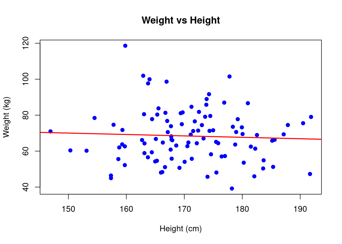
# Boxplot with formula
boxplot(weight ~ gender, data = df,
        main = "Weight by Gender",
        xlab = "Gender",
        ylab = "Weight (kg)",
        col = c("pink", "lightblue"))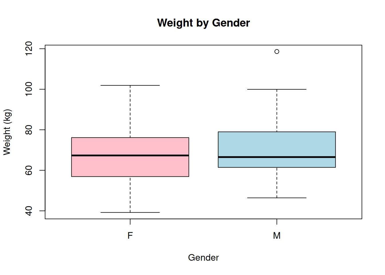
Example 2: ANOVA with Formulas
# Create categorical data
df$age_group <- cut(df$age, breaks = c(0, 30, 45, 100),
                     labels = c("Young", "Middle", "Senior"))

# One-way ANOVA
aov1 <- aov(weight ~ age_group, data = df)
summary(aov1)
Df Sum Sq Mean Sq F value Pr(>F)
age_group 2 305 152.5 0.721 0.489
Residuals 97 20523 211.6 # Two-way ANOVA with interaction
aov2 <- aov(weight ~ age_group * gender, data = df)
summary(aov2) Df Sum Sq Mean Sq F value Pr(>F)
age_group 2 305 152.52 0.718 0.490
gender 1 92 91.89 0.433 0.512
age_group:gender 2 471 235.51 1.109 0.334
Residuals 94 19961 212.35 Example 3: Data Manipulation with Formulas
# Aggregate function uses formulas
# Calculate mean weight by gender
aggregate(weight ~ gender, data = df, FUN = mean)
gender weight
1 F 67.47088
2 M 69.55251# Multiple variables
aggregate(cbind(weight, height) ~ gender + age_group, data = df, FUN = mean) gender age_group weight height
1 F Young 70.60824 172.8042
2 M Young 71.67341 172.5615
3 F Middle 65.43550 169.9501
4 M Middle 73.15206 168.0989
5 F Senior 67.69240 171.9951
6 M Senior 65.33892 170.4329Common Patterns and Shortcuts
No Intercept Models
# Remove intercept with -1 or +0
model13 <- lm(weight ~ height - 1, data = df)
model14 <- lm(weight ~ height + 0, data = df)
Update Formula
# Update an existing model
model_updated <- update(model2, . ~ . + gender)
# Adds gender to the existing formula

# Remove a term
model_updated2 <- update(model2, . ~ . - age)
Complex Interactions
# Three-way interaction
model15 <- lm(weight ~ height * age * gender, data = df)

# Specific interaction structure
model16 <- lm(weight ~ height + age + height:age + gender, data = df)
Formula Cheat Sheet
| Operator | Meaning | Example |
|---|---|---|
~ |
“modeled by” | y ~ x |
+ |
Include term | y ~ x + z |
- |
Exclude term | y ~ . - x |
: |
Interaction only | y ~ x:z |
* |
Main effects + interaction | y ~ x * z equals y ~ x + z + x:z |
. |
All other variables | y ~ . |
^ |
Interactions to degree | y ~ (x + z)^2 |
I() |
As-is arithmetic | y ~ I(x^2) |
-1 or +0 |
Remove intercept | y ~ x - 1 |
1 |
Intercept only | y ~ 1 |
Tips for Success
- Start simple: Begin with basic formulas and add complexity as needed
- Check expansions: Use
model.matrix()to see how your formula expands - Name clearly: Use descriptive variable names to make formulas readable
- Test interactions: Always examine whether interactions improve your model
- Read the docs: Different packages may interpret formulas slightly differently
# See how formula expands to design matrix
head(model.matrix(weight ~ height * gender, data = df))
(Intercept) height genderM height:genderM
1 1 164.3952 0 0.0000
2 1 167.6982 0 0.0000
3 1 185.5871 1 185.5871
4 1 170.7051 0 0.0000
5 1 171.2929 1 171.2929
6 1 187.1506 0 0.0000Conclusion
R’s formula syntax is a powerful and elegant way to specify statistical models and data relationships. While it has a learning curve, mastering formulas will make your R code more concise and expressive. Practice with real data, and soon the notation will become second nature!
Additional Resources
- R Documentation:
?formula - Model specification:
?lm,?glm,?aov - Formula tutorial:
vignette("formula")in various packages - Advanced modeling: Check packages like
lme4,mgcv, andnlmefor more complex formula applications
sessionInfo()R version 4.5.0 (2025-04-11)
Platform: x86_64-pc-linux-gnu
Running under: Ubuntu 24.04.3 LTS
Matrix products: default
BLAS: /usr/lib/x86_64-linux-gnu/openblas-pthread/libblas.so.3
LAPACK: /usr/lib/x86_64-linux-gnu/openblas-pthread/libopenblasp-r0.3.26.so; LAPACK version 3.12.0
locale:
[1] LC_CTYPE=en_US.UTF-8 LC_NUMERIC=C
[3] LC_TIME=en_US.UTF-8 LC_COLLATE=en_US.UTF-8
[5] LC_MONETARY=en_US.UTF-8 LC_MESSAGES=en_US.UTF-8
[7] LC_PAPER=en_US.UTF-8 LC_NAME=C
[9] LC_ADDRESS=C LC_TELEPHONE=C
[11] LC_MEASUREMENT=en_US.UTF-8 LC_IDENTIFICATION=C
time zone: Etc/UTC
tzcode source: system (glibc)
attached base packages:
[1] stats graphics grDevices utils datasets methods base
other attached packages:
[1] lubridate_1.9.4 forcats_1.0.0 stringr_1.5.1 dplyr_1.1.4
[5] purrr_1.0.4 readr_2.1.5 tidyr_1.3.1 tibble_3.3.0
[9] ggplot2_3.5.2 tidyverse_2.0.0 workflowr_1.7.1
loaded via a namespace (and not attached):
[1] sass_0.4.10 generics_0.1.4 stringi_1.8.7 hms_1.1.3
[5] digest_0.6.37 magrittr_2.0.3 timechange_0.3.0 evaluate_1.0.3
[9] grid_4.5.0 RColorBrewer_1.1-3 fastmap_1.2.0 rprojroot_2.0.4
[13] jsonlite_2.0.0 processx_3.8.6 whisker_0.4.1 ps_1.9.1
[17] promises_1.3.3 httr_1.4.7 scales_1.4.0 jquerylib_0.1.4
[21] cli_3.6.5 rlang_1.1.6 withr_3.0.2 cachem_1.1.0
[25] yaml_2.3.10 tools_4.5.0 tzdb_0.5.0 httpuv_1.6.16
[29] vctrs_0.6.5 R6_2.6.1 lifecycle_1.0.4 git2r_0.36.2
[33] fs_1.6.6 pkgconfig_2.0.3 callr_3.7.6 pillar_1.10.2
[37] bslib_0.9.0 later_1.4.2 gtable_0.3.6 glue_1.8.0
[41] Rcpp_1.0.14 xfun_0.52 tidyselect_1.2.1 rstudioapi_0.17.1
[45] knitr_1.50 farver_2.1.2 htmltools_0.5.8.1 rmarkdown_2.29
[49] compiler_4.5.0 getPass_0.2-4