Introduction to the Fourier Transform
2026-02-02
Last updated: 2026-02-02
Checks: 7 0
Knit directory: muse/
This reproducible R Markdown analysis was created with workflowr (version 1.7.1). The Checks tab describes the reproducibility checks that were applied when the results were created. The Past versions tab lists the development history.
Great! Since the R Markdown file has been committed to the Git repository, you know the exact version of the code that produced these results.
Great job! The global environment was empty. Objects defined in the global environment can affect the analysis in your R Markdown file in unknown ways. For reproduciblity it’s best to always run the code in an empty environment.
The command set.seed(20200712) was run prior to running
the code in the R Markdown file. Setting a seed ensures that any results
that rely on randomness, e.g. subsampling or permutations, are
reproducible.
Great job! Recording the operating system, R version, and package versions is critical for reproducibility.
Nice! There were no cached chunks for this analysis, so you can be confident that you successfully produced the results during this run.
Great job! Using relative paths to the files within your workflowr project makes it easier to run your code on other machines.
Great! You are using Git for version control. Tracking code development and connecting the code version to the results is critical for reproducibility.
The results in this page were generated with repository version 070a399. See the Past versions tab to see a history of the changes made to the R Markdown and HTML files.
Note that you need to be careful to ensure that all relevant files for
the analysis have been committed to Git prior to generating the results
(you can use wflow_publish or
wflow_git_commit). workflowr only checks the R Markdown
file, but you know if there are other scripts or data files that it
depends on. Below is the status of the Git repository when the results
were generated:
Ignored files:
    Ignored:    .Rproj.user/
    Ignored:    data/1M_neurons_filtered_gene_bc_matrices_h5.h5
    Ignored:    data/293t/
    Ignored:    data/293t_3t3_filtered_gene_bc_matrices.tar.gz
    Ignored:    data/293t_filtered_gene_bc_matrices.tar.gz
    Ignored:    data/5k_Human_Donor1_PBMC_3p_gem-x_5k_Human_Donor1_PBMC_3p_gem-x_count_sample_filtered_feature_bc_matrix.h5
    Ignored:    data/5k_Human_Donor2_PBMC_3p_gem-x_5k_Human_Donor2_PBMC_3p_gem-x_count_sample_filtered_feature_bc_matrix.h5
    Ignored:    data/5k_Human_Donor3_PBMC_3p_gem-x_5k_Human_Donor3_PBMC_3p_gem-x_count_sample_filtered_feature_bc_matrix.h5
    Ignored:    data/5k_Human_Donor4_PBMC_3p_gem-x_5k_Human_Donor4_PBMC_3p_gem-x_count_sample_filtered_feature_bc_matrix.h5
    Ignored:    data/97516b79-8d08-46a6-b329-5d0a25b0be98.h5ad
    Ignored:    data/Parent_SC3v3_Human_Glioblastoma_filtered_feature_bc_matrix.tar.gz
    Ignored:    data/brain_counts/
    Ignored:    data/cl.obo
    Ignored:    data/cl.owl
    Ignored:    data/jurkat/
    Ignored:    data/jurkat:293t_50:50_filtered_gene_bc_matrices.tar.gz
    Ignored:    data/jurkat_293t/
    Ignored:    data/jurkat_filtered_gene_bc_matrices.tar.gz
    Ignored:    data/pbmc20k/
    Ignored:    data/pbmc20k_seurat/
    Ignored:    data/pbmc3k.csv
    Ignored:    data/pbmc3k.csv.gz
    Ignored:    data/pbmc3k.h5ad
    Ignored:    data/pbmc3k/
    Ignored:    data/pbmc3k_bpcells_mat/
    Ignored:    data/pbmc3k_export.mtx
    Ignored:    data/pbmc3k_matrix.mtx
    Ignored:    data/pbmc3k_seurat.rds
    Ignored:    data/pbmc4k_filtered_gene_bc_matrices.tar.gz
    Ignored:    data/pbmc_1k_v3_filtered_feature_bc_matrix.h5
    Ignored:    data/pbmc_1k_v3_raw_feature_bc_matrix.h5
    Ignored:    data/refdata-gex-GRCh38-2020-A.tar.gz
    Ignored:    data/seurat_1m_neuron.rds
    Ignored:    data/t_3k_filtered_gene_bc_matrices.tar.gz
    Ignored:    r_packages_4.4.1/
    Ignored:    r_packages_4.5.0/

Untracked files:
    Untracked:  .claude/
    Untracked:  CLAUDE.md
    Untracked:  analysis/bioc.Rmd
    Untracked:  analysis/bioc_scrnaseq.Rmd
    Untracked:  analysis/chick_weight.Rmd
    Untracked:  analysis/likelihood.Rmd
    Untracked:  bpcells_matrix/
    Untracked:  data/Caenorhabditis_elegans.WBcel235.113.gtf.gz
    Untracked:  data/GCF_043380555.1-RS_2024_12_gene_ontology.gaf.gz
    Untracked:  data/arab.rds
    Untracked:  data/astronomicalunit.csv
    Untracked:  data/femaleMiceWeights.csv
    Untracked:  data/lung_bcell.rds
    Untracked:  m3/
    Untracked:  women.json

Unstaged changes:
    Modified:   analysis/isoform_switch_analyzer.Rmd
    Modified:   analysis/linear_models.Rmd
Note that any generated files, e.g. HTML, png, CSS, etc., are not included in this status report because it is ok for generated content to have uncommitted changes.
These are the previous versions of the repository in which changes were
made to the R Markdown (analysis/fourier_transform.Rmd) and
HTML (docs/fourier_transform.html) files. If you’ve
configured a remote Git repository (see ?wflow_git_remote),
click on the hyperlinks in the table below to view the files as they
were in that past version.
| File | Version | Author | Date | Message |
|---|---|---|---|---|
| Rmd | 070a399 | Dave Tang | 2026-02-02 | Introduction to the Fourier Transform |
What is the Fourier Transform?
The Fourier Transform is a mathematical technique that decomposes a signal into its constituent frequencies. Named after French mathematician Jean-Baptiste Joseph Fourier, it transforms data from the time domain (or spatial domain) into the frequency domain.
If you hear a musical chord (when you play three or more notes simultaneously to create a harmonic sound), the Fourier Transform can tell you which individual notes make up that chord and how loud each note is.
Why is it useful?
The Fourier Transform is fundamental in many fields:
- Signal processing: Filtering noise from audio or images
- Bioinformatics: Analysing periodic patterns in DNA sequences, spectroscopy data
- Image processing: JPEG compression, edge detection
- Physics: Quantum mechanics, optics, acoustics
The intuition
Any periodic signal can be represented as a sum of sine and cosine waves of different frequencies. The Fourier Transform finds the amplitude and phase of each frequency component.
Let’s start with a simple example: creating a signal from known frequencies.
- Hertz is a unit that measures frequency: how many times something happens per second.
- 100 Hz means something is happening 100 times per second.
# Create a time vector (1 second of data sampled at 100 Hz)
sample_rate <- 100
duration <- 1
t <- seq(0, duration, by = 1/sample_rate)

# Create a signal with two frequencies: 5 Hz and 20 Hz
freq1 <- 5
freq2 <- 20

signal <- sin(2 * pi * freq1 * t) + 0.5 * sin(2 * pi * freq2 * t)

plot(t, signal, type = "l",
     xlab = "Time (seconds)",
     ylab = "Amplitude",
     main = "Signal with 5 Hz and 20 Hz components")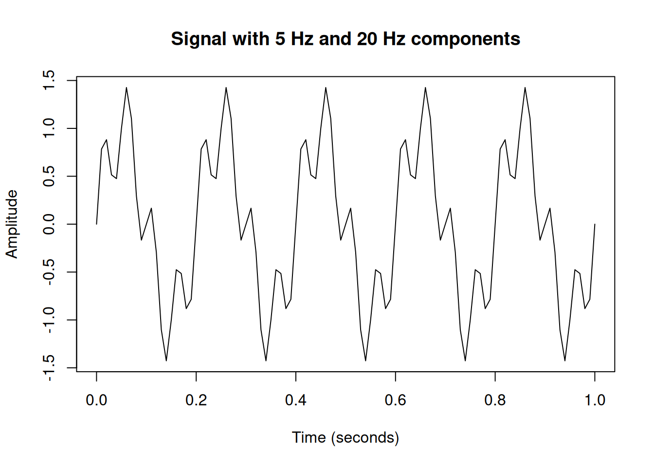
Looking at this signal, it’s not immediately obvious that it’s composed of two sine waves. Let’s use the Fourier Transform to reveal the hidden frequencies.
The Fast Fourier Transform (FFT) in R
R provides the fft() function which implements the Fast
Fourier Transform, an efficient algorithm for computing the Discrete
Fourier Transform (DFT).
# Compute the FFT
fft_result <- fft(signal)

# The FFT returns complex numbers
head(fft_result)
[1] -8.437695e-15+ 0.0000000i 7.025444e-03- 0.2257903i
[3] 3.167017e-02- 0.5084300i 9.109146e-02- 0.9733405i
[5] 2.734064e-01- 2.1861049i 7.768581e+00-49.5475020iThe FFT returns complex numbers. The magnitude (absolute value) tells us the amplitude of each frequency component. The phase (argument) tells us the phase shift.
# Calculate magnitude
magnitude <- Mod(fft_result)

# Create frequency axis
n <- length(signal)
freq <- (0:(n-1)) * sample_rate / n

# Plot only the first half (positive frequencies)
# The FFT output is symmetric for real signals
half_n <- floor(n/2)

plot(freq[1:half_n], magnitude[1:half_n], type = "h",
     xlab = "Frequency (Hz)",
     ylab = "Magnitude",
     main = "Frequency Spectrum")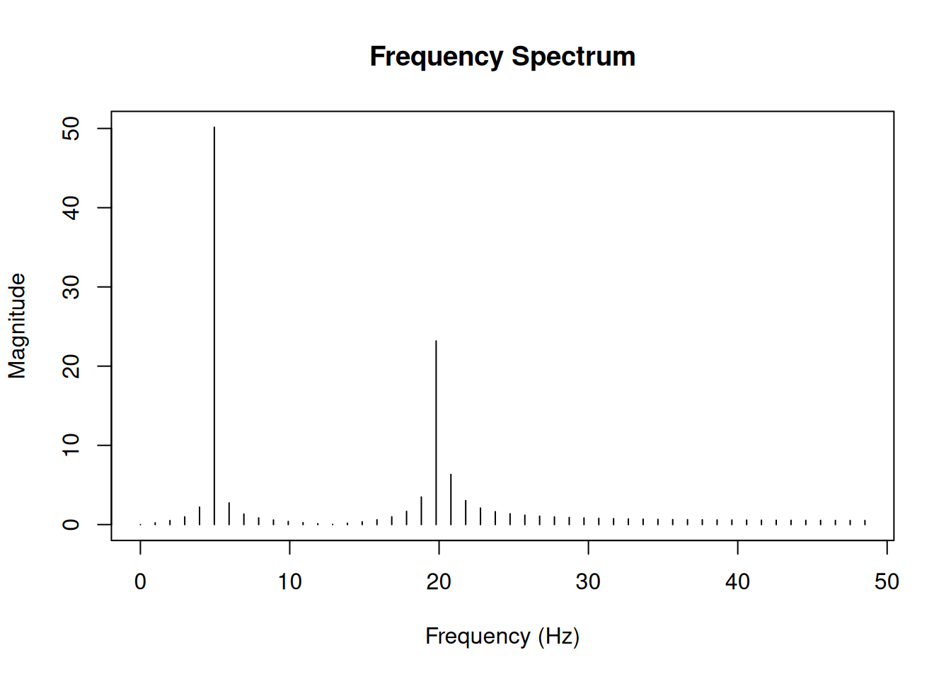
Notice the peaks at 5 Hz and 20 Hz - exactly the frequencies we used to create our signal! The peak at 5 Hz is twice as high as the peak at 20 Hz, reflecting the amplitude ratio (1.0 vs 0.5) in our original signal.
Normalising the FFT output
To get meaningful amplitude values, we need to normalise the FFT output.
# Normalise by the number of samples
# Multiply by 2 for single-sided spectrum (except DC component)
magnitude_normalised <- (2 * Mod(fft_result) / n)[1:half_n]
magnitude_normalised[1] <- magnitude_normalised[1] / 2  # DC component

plot(freq[1:half_n], magnitude_normalised, type = "h",
     xlab = "Frequency (Hz)",
     ylab = "Amplitude",
     main = "Normalised Frequency Spectrum")

# Add points to highlight peaks
abline(h = 0, col = "gray")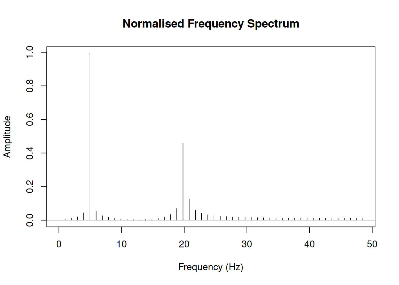
Now the amplitudes approximately match our original signal (1.0 for 5 Hz and 0.5 for 20 Hz).
A practical example: Removing noise
One common application is filtering noise from a signal. Let’s add noise to our signal and then filter it out.
# Add random noise
set.seed(42)
noisy_signal <- signal + rnorm(length(signal), sd = 0.5)

par(mfrow = c(2, 1), mar = c(4, 4, 2, 1))
plot(t, signal, type = "l",
     xlab = "Time (seconds)", ylab = "Amplitude",
     main = "Original Signal")
plot(t, noisy_signal, type = "l",
     xlab = "Time (seconds)", ylab = "Amplitude",
     main = "Noisy Signal")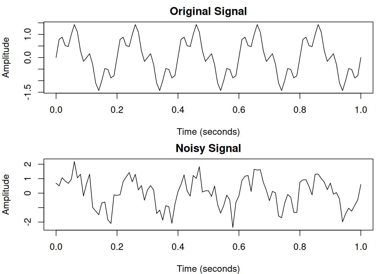
par(mfrow = c(1, 1))# FFT of noisy signal
fft_noisy <- fft(noisy_signal)
# Create a low-pass filter (keep frequencies below 25 Hz)
cutoff <- 25
filter_mask <- rep(0, n)
freq_indices <- which(freq <= cutoff | freq >= (sample_rate - cutoff))
filter_mask[freq_indices] <- 1
# Apply filter
fft_filtered <- fft_noisy * filter_mask
# Inverse FFT to get back to time domain
filtered_signal <- Re(fft(fft_filtered, inverse = TRUE) / n)
par(mfrow = c(2, 1), mar = c(4, 4, 2, 1))
plot(t, noisy_signal, type = "l", col = "gray",
xlab = "Time (seconds)", ylab = "Amplitude",
main = "Noisy vs Filtered Signal")
lines(t, filtered_signal, col = "blue", lwd = 2)
legend("topright", legend = c("Noisy", "Filtered"),
col = c("gray", "blue"), lty = 1, lwd = c(1, 2))
plot(t, signal, type = "l", col = "black",
xlab = "Time (seconds)", ylab = "Amplitude",
main = "Original vs Filtered Signal")
lines(t, filtered_signal, col = "blue", lwd = 2, lty = 2)
legend("topright", legend = c("Original", "Filtered"),
col = c("black", "blue"), lty = c(1, 2), lwd = c(1, 2))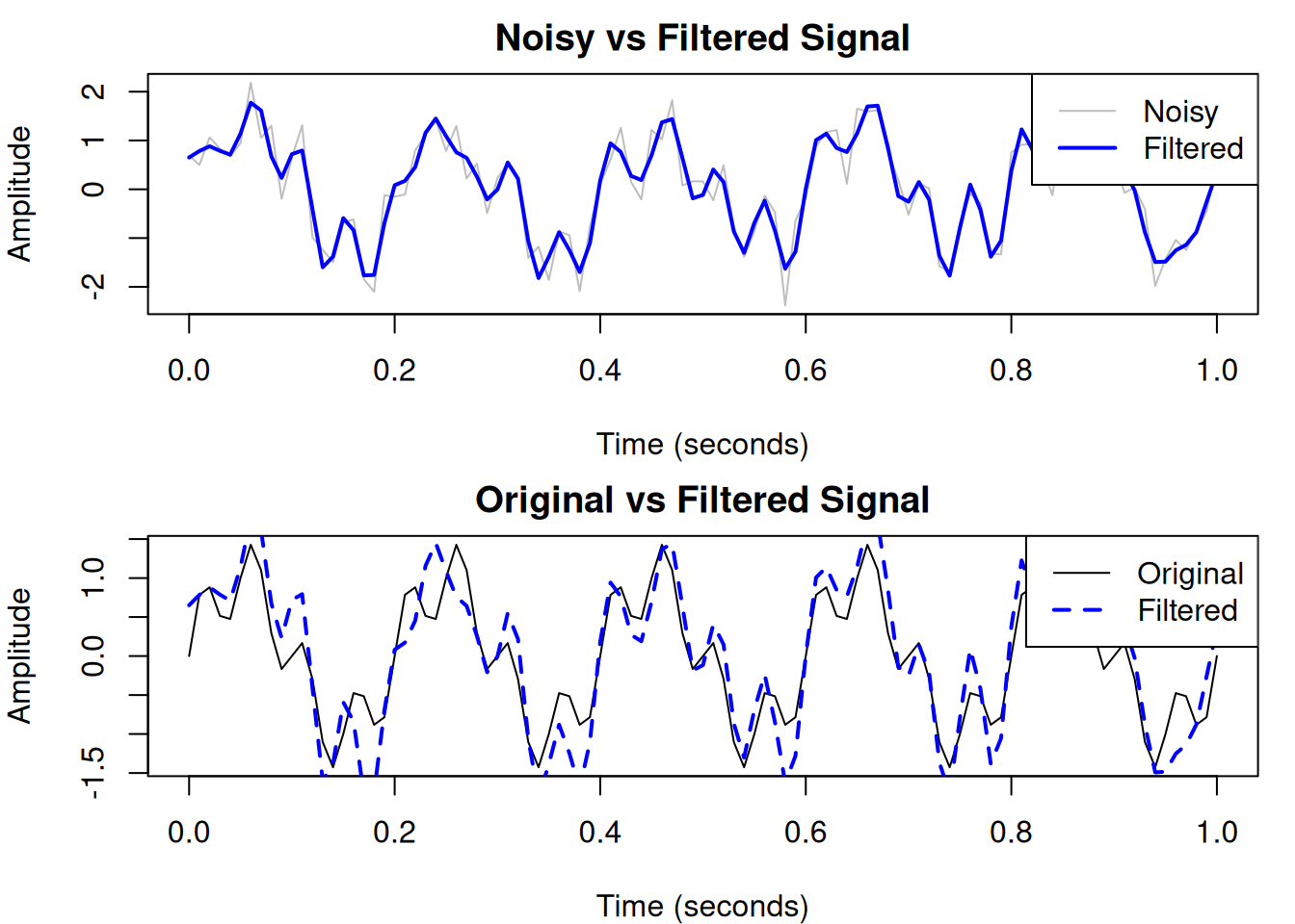
par(mfrow = c(1, 1))Understanding the mathematics
The Discrete Fourier Transform is defined as:
\[X_k = \sum_{n=0}^{N-1} x_n \cdot e^{-i 2\pi k n / N}\]
Where:
- \(x_n\) is the input signal at time point \(n\)
- \(X_k\) is the complex amplitude at frequency \(k\)
- \(N\) is the total number of samples
- \(e^{-i 2\pi k n / N}\) represents complex sinusoids (from Euler’s formula: \(e^{i\theta} = \cos\theta + i\sin\theta\))
The inverse transform reconstructs the original signal:
\[x_n = \frac{1}{N} \sum_{k=0}^{N-1} X_k \cdot e^{i 2\pi k n / N}\]
Computing DFT manually
Let’s verify our understanding by computing the DFT manually for a small signal.
# Simple signal
x <- c(1, 2, 3, 4)
N <- length(x)

# Manual DFT
manual_dft <- function(x) {
  N <- length(x)
  X <- complex(N)
  for (k in 0:(N-1)) {
    for (n in 0:(N-1)) {
      X[k+1] <- X[k+1] + x[n+1] * exp(-1i * 2 * pi * k * n / N)
    }
  }
  return(X)
}

# Compare manual vs fft()
manual_result <- manual_dft(x)
fft_result <- fft(x)

data.frame(
  k = 0:(N-1),
  manual_real = round(Re(manual_result), 6),
  manual_imag = round(Im(manual_result), 6),
  fft_real = round(Re(fft_result), 6),
  fft_imag = round(Im(fft_result), 6)
)
k manual_real manual_imag fft_real fft_imag
1 0 10 0 10 0
2 1 -2 2 -2 2
3 2 -2 0 -2 0
4 3 -2 -2 -2 -2The results match! The FFT is simply a faster algorithm (\(O(N \log N)\) vs \(O(N^2)\)) for computing the same thing.
Power spectrum
The power spectrum shows the distribution of signal power across frequencies. It’s computed as the squared magnitude of the FFT.
# Create a more complex signal
t_long <- seq(0, 2, by = 1/sample_rate)
complex_signal <- sin(2 * pi * 3 * t_long) +
                  0.7 * sin(2 * pi * 7 * t_long) +
                  0.3 * sin(2 * pi * 15 * t_long)

# Compute power spectrum
fft_complex <- fft(complex_signal)
n_long <- length(complex_signal)
power <- (Mod(fft_complex)^2) / n_long
freq_long <- (0:(n_long-1)) * sample_rate / n_long

# Plot
half_n_long <- floor(n_long/2)
plot(freq_long[1:half_n_long], power[1:half_n_long], type = "h",
     xlab = "Frequency (Hz)",
     ylab = "Power",
     main = "Power Spectrum")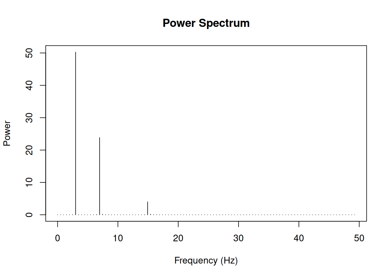
Summary
Key takeaways:
- The Fourier Transform converts signals from time domain to frequency domain
- Use
fft()in R for the Fast Fourier Transform - The FFT returns complex numbers; use
Mod()for magnitude,Arg()for phase - For real signals, the FFT output is symmetric - only the first half is needed
- Remember to normalise by dividing by the number of samples
sessionInfo()R version 4.5.0 (2025-04-11)
Platform: x86_64-pc-linux-gnu
Running under: Ubuntu 24.04.3 LTS
Matrix products: default
BLAS: /usr/lib/x86_64-linux-gnu/openblas-pthread/libblas.so.3
LAPACK: /usr/lib/x86_64-linux-gnu/openblas-pthread/libopenblasp-r0.3.26.so; LAPACK version 3.12.0
locale:
[1] LC_CTYPE=en_US.UTF-8 LC_NUMERIC=C
[3] LC_TIME=en_US.UTF-8 LC_COLLATE=en_US.UTF-8
[5] LC_MONETARY=en_US.UTF-8 LC_MESSAGES=en_US.UTF-8
[7] LC_PAPER=en_US.UTF-8 LC_NAME=C
[9] LC_ADDRESS=C LC_TELEPHONE=C
[11] LC_MEASUREMENT=en_US.UTF-8 LC_IDENTIFICATION=C
time zone: Etc/UTC
tzcode source: system (glibc)
attached base packages:
[1] stats graphics grDevices utils datasets methods base
other attached packages:
[1] workflowr_1.7.1
loaded via a namespace (and not attached):
[1] vctrs_0.6.5 httr_1.4.7 cli_3.6.5 knitr_1.50
[5] rlang_1.1.6 xfun_0.52 stringi_1.8.7 processx_3.8.6
[9] promises_1.3.3 jsonlite_2.0.0 glue_1.8.0 rprojroot_2.0.4
[13] git2r_0.36.2 htmltools_0.5.8.1 httpuv_1.6.16 ps_1.9.1
[17] sass_0.4.10 rmarkdown_2.29 jquerylib_0.1.4 tibble_3.3.0
[21] evaluate_1.0.3 fastmap_1.2.0 yaml_2.3.10 lifecycle_1.0.4
[25] whisker_0.4.1 stringr_1.5.1 compiler_4.5.0 fs_1.6.6
[29] pkgconfig_2.0.3 Rcpp_1.0.14 rstudioapi_0.17.1 later_1.4.2
[33] digest_0.6.37 R6_2.6.1 pillar_1.10.2 callr_3.7.6
[37] magrittr_2.0.3 bslib_0.9.0 tools_4.5.0 cachem_1.1.0
[41] getPass_0.2-4