Visualising Google Trends results with R
2020-11-10
Last updated: 2020-11-10
Checks: 7 0
Knit directory: muse/
This reproducible R Markdown analysis was created with workflowr (version 1.6.2). The Checks tab describes the reproducibility checks that were applied when the results were created. The Past versions tab lists the development history.
Great! Since the R Markdown file has been committed to the Git repository, you know the exact version of the code that produced these results.
Great job! The global environment was empty. Objects defined in the global environment can affect the analysis in your R Markdown file in unknown ways. For reproduciblity it’s best to always run the code in an empty environment.
The command set.seed(20200712) was run prior to running the code in the R Markdown file. Setting a seed ensures that any results that rely on randomness, e.g. subsampling or permutations, are reproducible.
Great job! Recording the operating system, R version, and package versions is critical for reproducibility.
Nice! There were no cached chunks for this analysis, so you can be confident that you successfully produced the results during this run.
Great job! Using relative paths to the files within your workflowr project makes it easier to run your code on other machines.
Great! You are using Git for version control. Tracking code development and connecting the code version to the results is critical for reproducibility.
The results in this page were generated with repository version 268312f. See the Past versions tab to see a history of the changes made to the R Markdown and HTML files.
Note that you need to be careful to ensure that all relevant files for the analysis have been committed to Git prior to generating the results (you can use wflow_publish or wflow_git_commit). workflowr only checks the R Markdown file, but you know if there are other scripts or data files that it depends on. Below is the status of the Git repository when the results were generated:
Ignored files:
    Ignored:    .Rhistory
    Ignored:    .Rproj.user/
    Ignored:    analysis/.Rhistory

Untracked files:
    Untracked:  analysis/linear_regression.Rmd
Note that any generated files, e.g. HTML, png, CSS, etc., are not included in this status report because it is ok for generated content to have uncommitted changes.
These are the previous versions of the repository in which changes were made to the R Markdown (analysis/google_trends.Rmd) and HTML (docs/google_trends.html) files. If you’ve configured a remote Git repository (see ?wflow_git_remote), click on the hyperlinks in the table below to view the files as they were in that past version.
| File | Version | Author | Date | Message |
|---|---|---|---|---|
| Rmd | 268312f | davetang | 2020-11-10 | wflow_publish(files = c(“analysis/index.Rmd”, “analysis/google_trends.Rmd”, |
This post is on plotting Google Trends results with R. If you have never heard of or used Google Trends, it’s fun! You can see how certain keywords have trended over the years and have the results broken down into regions and countries. In this post, I will use the gtrendsR package to perform Google Trends searches with R and demonstrate how to plot the data that is returned.
To get started, install the gtrendsR, dplyr, ggplot2, and maps packages (if you haven’t already).
install.packages("gtrendsR", "dplyr", "ggplot2", "maps")The gtrends function performs the search. The function has several parameters; I have set geo to focus on the United States and time to include all results since the beginning of Google Trends (2004). I like the San Antonio Spurs, so that will be the keyword for this example.
res <- gtrends("san antonio spurs",
               geo = "US",
               time = "all")

names(res)
[1] "interest_over_time" "interest_by_country" "interest_by_region"
[4] "interest_by_dma" "interest_by_city" "related_topics"
[7] "related_queries" The results are stored in a list that have self-explanatory names. I picked a keyword that should be region- and city-specific. Below I show the interest in “san antonio spurs” stratified by region, city, and DMA and sorted by the interest (highest to lowest).
res$interest_by_region %>%
  arrange(desc(hits)) %>%
  head(3)
location hits keyword geo gprop
1 Texas 100 san antonio spurs US web
2 New Mexico 25 san antonio spurs US web
3 Oklahoma 19 san antonio spurs US webres$interest_by_city %>%
arrange(desc(hits)) %>%
head(3) location hits keyword geo gprop
1 San Antonio 100 san antonio spurs US web
2 Canyon Lake 63 san antonio spurs US web
3 Laredo 56 san antonio spurs US webres$interest_by_dma %>%
arrange(desc(hits)) %>%
head(3) location hits keyword geo gprop
1 Tyler-Longview(Lufkin & Nacogdoches) TX 8 san antonio spurs US web
2 Dallas-Ft. Worth TX 7 san antonio spurs US web
3 Wichita Falls TX & Lawton OK 7 san antonio spurs US webI modified the plotting function from the gtrendsR package, so that the function just returns a ggplot object without plotting it, in order to customise the plot.
plot.gtrends.silent <- function(x, ...) {
  df <- x$interest_over_time
  df$date <- as.Date(df$date)
  df$hits <- if(typeof(df$hits) == 'character'){
    as.numeric(gsub('<','',df$hits))
    } else {
    df$hits
    }

  df$legend <- paste(df$keyword, " (", df$geo, ")", sep = "")

  p <- ggplot(df, aes_string(x = "date", y = "hits", color = "legend")) +
    geom_line() +
    xlab("Date") +
    ylab("Search hits") +
    ggtitle("Interest over time") +
    theme_bw() +
    theme(legend.title = element_blank())

  invisible(p)
}

my_plot <- plot.gtrends.silent(res)

my_plot +
  scale_x_date(date_breaks = "1 year", date_labels = "%Y") +
  theme(legend.position = "none")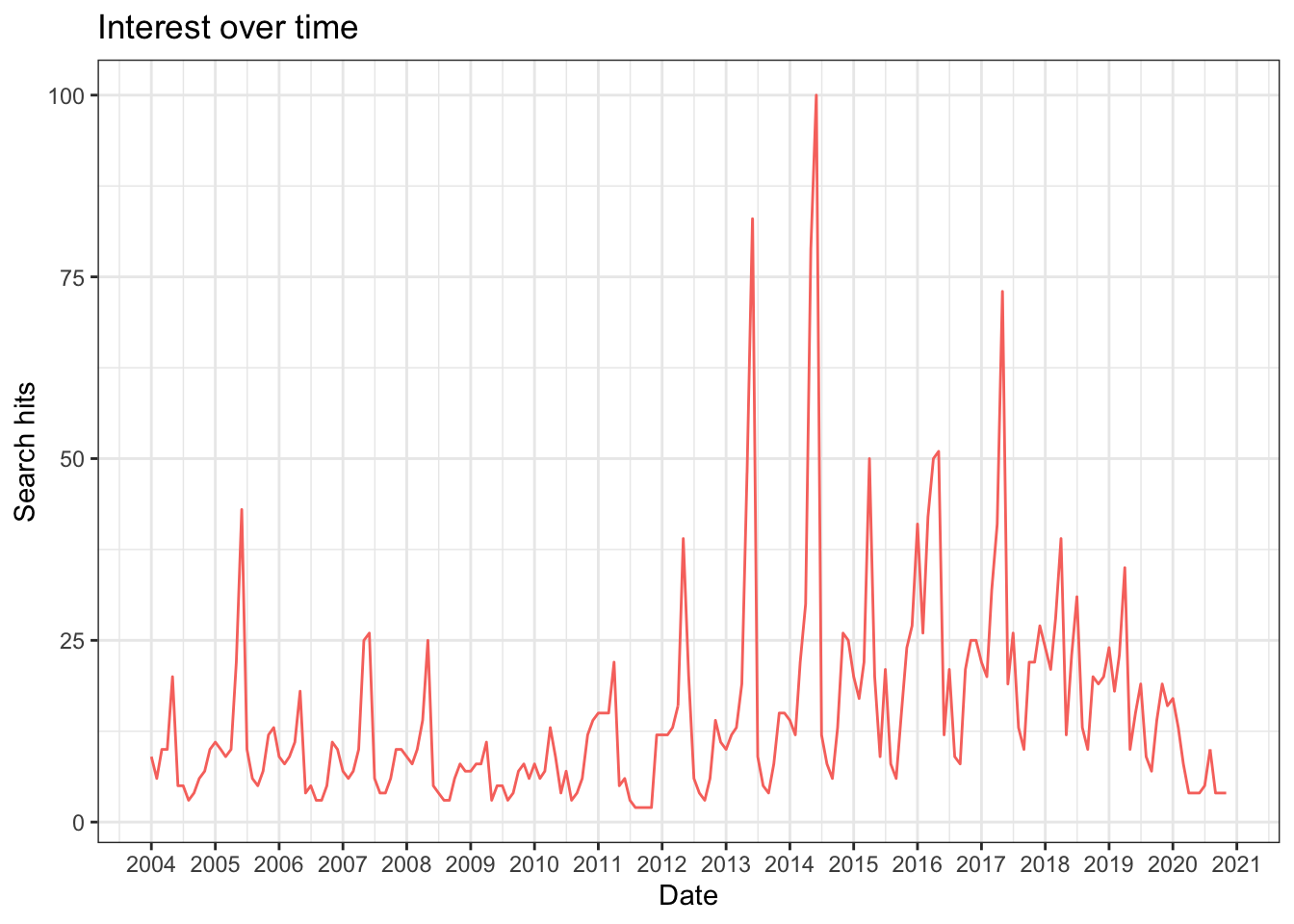
The seasonal trend is due to when the NBA season starts and ends. The spike in 2014 is when the San Antonio Spurs were the NBA champions; the spike in 2013 is when they reached the NBA finals but lost.
Next, I will show how to plot interest per country; I will colour each city by the interest of a certain keyword. I will use the map_data function to obtain coordinates (and polygon drawing groups and orders) of cities in the world as a data frame. In the first example, I will use the keyword “wantok”, which means a close friend in Tok Pisin; this is the main language spoken in Papua New Guinea, the country I grew up in.
world <- map_data("world")

# change the region names to match the region names returned by Google Trends
world %>%
  mutate(region = replace(region, region=="USA", "United States")) %>%
  mutate(region = replace(region, region=="UK", "United Kingdom")) -> world

# perform search
res_world <- gtrends("wantok", time = "all")

# create data frame for plotting
res_world$interest_by_country %>%
  filter(location %in% world$region, hits > 0) %>%
  mutate(region = location, hits = as.numeric(hits)) %>%
  select(region, hits) -> my_df

ggplot() +
  geom_map(data = world,
           map = world,
           aes(x = long, y = lat, map_id = region),
           fill="#ffffff", color="#ffffff", size=0.15) +
  geom_map(data = my_df,
           map = world,
           aes(fill = hits, map_id = region),
           color="#ffffff", size=0.15) +
  scale_fill_continuous(low = 'grey', high = 'red') +
  theme(axis.ticks = element_blank(),
        axis.text = element_blank(),
        axis.title = element_blank())
Warning: Ignoring unknown aesthetics: x, y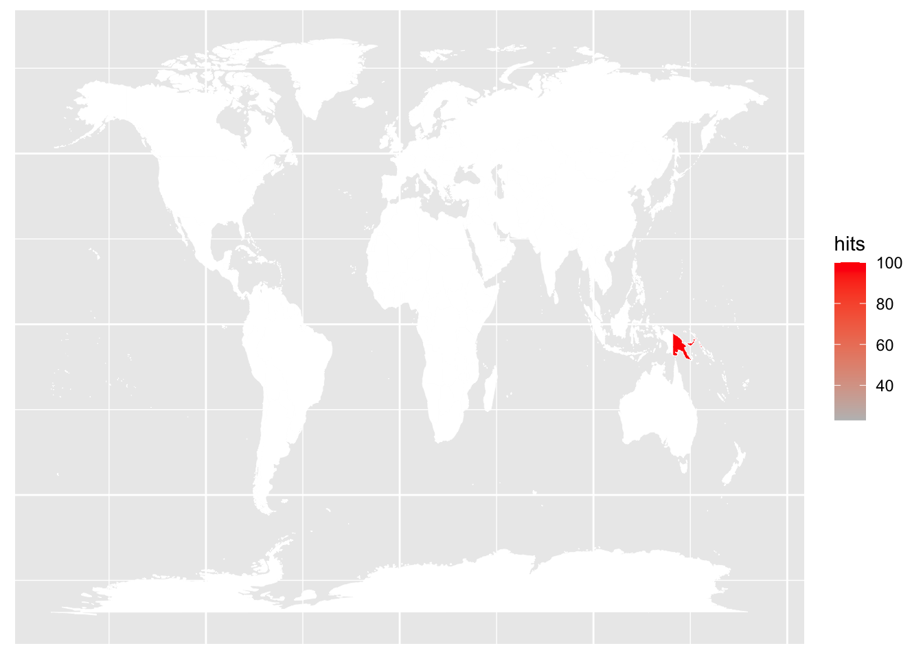
As expected, the top interest in the keyword “wantok” is in Papua New Guinea.
We can also only focus on the United States. Here I will use the keyword “swamp gravy”, which was something I learned about while listening to the Planet Money podcast (which I highly recommend).
res <- gtrends("swamp gravy",
               geo = "US",
               time = "all")

state <- map_data("state")

res$interest_by_region %>%
  mutate(region = tolower(location)) %>%
  filter(region %in% state$region) %>%
  select(region, hits) -> my_df

ggplot() +
  geom_map(data = state,
           map = state,
           aes(x = long, y = lat, map_id = region),
           fill="#ffffff", color="#ffffff", size=0.15) +
  geom_map(data = my_df,
           map = state,
           aes(fill = hits, map_id = region),
           color="#ffffff", size=0.15) +
  scale_fill_continuous(low = 'grey', high = 'red') +
  theme(panel.background = element_blank(),
        axis.ticks = element_blank(),
        axis.text = element_blank(),
        axis.title = element_blank())
Warning: Ignoring unknown aesthetics: x, y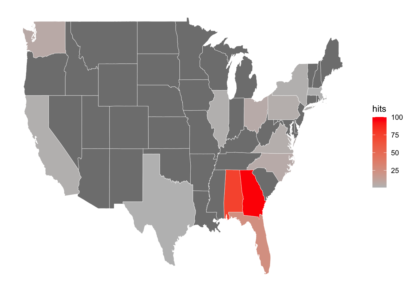
Swamp gravy is a play that has become the U.S. state of Georgia’s official folk-life play. The state of Georgia (and its neighbouring state Alabama) indeed has the highest interest in the keyword.
Since this is a bioinformatics blog, I will show results for the keyword “bioinformatics”.
res <- gtrends("bioinformatics",
               geo = "US",
               time = "all")

state <- map_data("state")

res$interest_by_region %>%
  mutate(region = tolower(location)) %>%
  filter(region %in% state$region) %>%
  select(region, hits) -> my_df

ggplot() +
  geom_map(data = state,
           map = state,
           aes(x = long, y = lat, map_id = region),
           fill="#ffffff", color="#ffffff", size=0.15) +
  geom_map(data = my_df,
           map = state,
           aes(fill = hits, map_id = region),
           color="#ffffff", size=0.15) +
  scale_fill_continuous(low = 'grey', high = 'red') +
  theme(panel.background = element_blank(),
        axis.ticks = element_blank(),
        axis.text = element_blank(),
        axis.title = element_blank())
Warning: Ignoring unknown aesthetics: x, y
Maryland (location of the NIH) and Massachusetts (location of the Broad Institute and various biotech startups) have the highest interest in bioinformatics.
Note that the US plots are missing Alaska and Hawaii and this is because these states are missing from the “state” map.
unique(map_data("state")$region) [1] "alabama" "arizona" "arkansas"
[4] "california" "colorado" "connecticut"
[7] "delaware" "district of columbia" "florida"
[10] "georgia" "idaho" "illinois"
[13] "indiana" "iowa" "kansas"
[16] "kentucky" "louisiana" "maine"
[19] "maryland" "massachusetts" "michigan"
[22] "minnesota" "mississippi" "missouri"
[25] "montana" "nebraska" "nevada"
[28] "new hampshire" "new jersey" "new mexico"
[31] "new york" "north carolina" "north dakota"
[34] "ohio" "oklahoma" "oregon"
[37] "pennsylvania" "rhode island" "south carolina"
[40] "south dakota" "tennessee" "texas"
[43] "utah" "vermont" "virginia"
[46] "washington" "west virginia" "wisconsin"
[49] "wyoming"
sessionInfo()R version 4.0.2 (2020-06-22)
Platform: x86_64-apple-darwin17.0 (64-bit)
Running under: macOS Catalina 10.15.7
Matrix products: default
BLAS: /Library/Frameworks/R.framework/Versions/4.0/Resources/lib/libRblas.dylib
LAPACK: /Library/Frameworks/R.framework/Versions/4.0/Resources/lib/libRlapack.dylib
locale:
[1] en_AU.UTF-8/en_AU.UTF-8/en_AU.UTF-8/C/en_AU.UTF-8/en_AU.UTF-8
attached base packages:
[1] stats graphics grDevices utils datasets methods base
other attached packages:
[1] maps_3.3.0 gtrendsR_1.4.7 forcats_0.5.0 stringr_1.4.0
[5] dplyr_1.0.2 purrr_0.3.4 readr_1.3.1 tidyr_1.1.2
[9] tibble_3.0.3 ggplot2_3.3.2 tidyverse_1.3.0 workflowr_1.6.2
loaded via a namespace (and not attached):
[1] tidyselect_1.1.0 xfun_0.16 haven_2.3.1 colorspace_1.4-1
[5] vctrs_0.3.4 generics_0.0.2 htmltools_0.5.0 yaml_2.2.1
[9] blob_1.2.1 rlang_0.4.7 later_1.1.0.1 pillar_1.4.6
[13] withr_2.2.0 glue_1.4.2 DBI_1.1.0 dbplyr_1.4.4
[17] modelr_0.1.8 readxl_1.3.1 lifecycle_0.2.0 munsell_0.5.0
[21] gtable_0.3.0 cellranger_1.1.0 rvest_0.3.6 evaluate_0.14
[25] labeling_0.3 knitr_1.29 httpuv_1.5.4 curl_4.3
[29] fansi_0.4.1 broom_0.7.0 Rcpp_1.0.5 promises_1.1.1
[33] backports_1.1.9 scales_1.1.1 jsonlite_1.7.0 farver_2.0.3
[37] fs_1.5.0 hms_0.5.3 digest_0.6.25 stringi_1.4.6
[41] rprojroot_1.3-2 grid_4.0.2 cli_2.0.2 tools_4.0.2
[45] magrittr_1.5 crayon_1.3.4 whisker_0.4 pkgconfig_2.0.3
[49] ellipsis_0.3.1 xml2_1.3.2 reprex_0.3.0 lubridate_1.7.9
[53] assertthat_0.2.1 rmarkdown_2.3 httr_1.4.2 rstudioapi_0.11
[57] R6_2.4.1 git2r_0.27.1 compiler_4.0.2