Linear Models for Microarray and Omics Data
2026-01-28
Last updated: 2026-01-28
Checks: 7 0
Knit directory: muse/
This reproducible R Markdown analysis was created with workflowr (version 1.7.1). The Checks tab describes the reproducibility checks that were applied when the results were created. The Past versions tab lists the development history.
Great! Since the R Markdown file has been committed to the Git repository, you know the exact version of the code that produced these results.
Great job! The global environment was empty. Objects defined in the global environment can affect the analysis in your R Markdown file in unknown ways. For reproduciblity it’s best to always run the code in an empty environment.
The command set.seed(20200712) was run prior to running
the code in the R Markdown file. Setting a seed ensures that any results
that rely on randomness, e.g. subsampling or permutations, are
reproducible.
Great job! Recording the operating system, R version, and package versions is critical for reproducibility.
Nice! There were no cached chunks for this analysis, so you can be confident that you successfully produced the results during this run.
Great job! Using relative paths to the files within your workflowr project makes it easier to run your code on other machines.
Great! You are using Git for version control. Tracking code development and connecting the code version to the results is critical for reproducibility.
The results in this page were generated with repository version 1e1a825. See the Past versions tab to see a history of the changes made to the R Markdown and HTML files.
Note that you need to be careful to ensure that all relevant files for
the analysis have been committed to Git prior to generating the results
(you can use wflow_publish or
wflow_git_commit). workflowr only checks the R Markdown
file, but you know if there are other scripts or data files that it
depends on. Below is the status of the Git repository when the results
were generated:
Ignored files:
    Ignored:    .Rproj.user/
    Ignored:    data/1M_neurons_filtered_gene_bc_matrices_h5.h5
    Ignored:    data/293t/
    Ignored:    data/293t_3t3_filtered_gene_bc_matrices.tar.gz
    Ignored:    data/293t_filtered_gene_bc_matrices.tar.gz
    Ignored:    data/5k_Human_Donor1_PBMC_3p_gem-x_5k_Human_Donor1_PBMC_3p_gem-x_count_sample_filtered_feature_bc_matrix.h5
    Ignored:    data/5k_Human_Donor2_PBMC_3p_gem-x_5k_Human_Donor2_PBMC_3p_gem-x_count_sample_filtered_feature_bc_matrix.h5
    Ignored:    data/5k_Human_Donor3_PBMC_3p_gem-x_5k_Human_Donor3_PBMC_3p_gem-x_count_sample_filtered_feature_bc_matrix.h5
    Ignored:    data/5k_Human_Donor4_PBMC_3p_gem-x_5k_Human_Donor4_PBMC_3p_gem-x_count_sample_filtered_feature_bc_matrix.h5
    Ignored:    data/97516b79-8d08-46a6-b329-5d0a25b0be98.h5ad
    Ignored:    data/Parent_SC3v3_Human_Glioblastoma_filtered_feature_bc_matrix.tar.gz
    Ignored:    data/brain_counts/
    Ignored:    data/cl.obo
    Ignored:    data/cl.owl
    Ignored:    data/jurkat/
    Ignored:    data/jurkat:293t_50:50_filtered_gene_bc_matrices.tar.gz
    Ignored:    data/jurkat_293t/
    Ignored:    data/jurkat_filtered_gene_bc_matrices.tar.gz
    Ignored:    data/pbmc20k/
    Ignored:    data/pbmc20k_seurat/
    Ignored:    data/pbmc3k.csv
    Ignored:    data/pbmc3k.csv.gz
    Ignored:    data/pbmc3k.h5ad
    Ignored:    data/pbmc3k/
    Ignored:    data/pbmc3k_bpcells_mat/
    Ignored:    data/pbmc3k_export.mtx
    Ignored:    data/pbmc3k_matrix.mtx
    Ignored:    data/pbmc3k_seurat.rds
    Ignored:    data/pbmc4k_filtered_gene_bc_matrices.tar.gz
    Ignored:    data/pbmc_1k_v3_filtered_feature_bc_matrix.h5
    Ignored:    data/pbmc_1k_v3_raw_feature_bc_matrix.h5
    Ignored:    data/refdata-gex-GRCh38-2020-A.tar.gz
    Ignored:    data/seurat_1m_neuron.rds
    Ignored:    data/t_3k_filtered_gene_bc_matrices.tar.gz
    Ignored:    r_packages_4.4.1/
    Ignored:    r_packages_4.5.0/

Untracked files:
    Untracked:  analysis/bioc.Rmd
    Untracked:  analysis/bioc_scrnaseq.Rmd
    Untracked:  analysis/likelihood.Rmd
    Untracked:  bpcells_matrix/
    Untracked:  data/Caenorhabditis_elegans.WBcel235.113.gtf.gz
    Untracked:  data/GCF_043380555.1-RS_2024_12_gene_ontology.gaf.gz
    Untracked:  data/arab.rds
    Untracked:  data/astronomicalunit.csv
    Untracked:  data/femaleMiceWeights.csv
    Untracked:  data/lung_bcell.rds
    Untracked:  m3/
    Untracked:  women.json

Unstaged changes:
    Modified:   analysis/icc.Rmd
    Modified:   analysis/isoform_switch_analyzer.Rmd
    Modified:   analysis/linear_models.Rmd
Note that any generated files, e.g. HTML, png, CSS, etc., are not included in this status report because it is ok for generated content to have uncommitted changes.
These are the previous versions of the repository in which changes were
made to the R Markdown (analysis/limma.Rmd) and HTML
(docs/limma.html) files. If you’ve configured a remote Git
repository (see ?wflow_git_remote), click on the hyperlinks
in the table below to view the files as they were in that past version.
| File | Version | Author | Date | Message |
|---|---|---|---|---|
| Rmd | 1e1a825 | Dave Tang | 2026-01-28 | Understanding limma |
Introduction
- Understand basic linear models and how they’re represented mathematically
- Learn about design matrices and how they encode experimental conditions
- Understand contrast matrices and how they specify comparisons of interest
- See how limma uses linear models for microarray and RNA-seq data
- Understand how edgeR uses generalized linear models for count data
- Learn the practical application of these concepts in differential expression analysis
Linear Model
A linear model is a statistical model that assumes a linear relationship between:
- Response variable, also known as, dependent variable, \(y\)
- Predictor variables, also known as independent variables, explanatory variables, \(x_1, x_2, ..., x_p\)
The general form of a linear model is:
\[ y = \beta_0 + \beta_1 x_1 + \beta_2 x_2 + ... + \beta_p x_p + \varepsilon \]
Where:
- \(y\) is the response variable (what we’re trying to explain)
- \(\beta_0\) is the intercept
- \(\beta_1, ..., \beta_p\) are coefficients (parameters we estimate)
- \(x_1, ..., x_p\) are predictor variables
- \(\varepsilon\) is the error term (residual), assumed to be normally distributed
Simple Linear Regression
Let’s start with the simplest case: one predictor variable.
set.seed(1984)
x <- 1:20
y <- 2 + 3*x + rnorm(20, 0, 5)  # y = 2 + 3*x + noise

model1 <- lm(y ~ x)
summary(model1)
Call:
lm(formula = y ~ x)

Residuals:
     Min       1Q   Median       3Q      Max
-10.6578  -3.3266   0.9095   3.5601   8.6517

Coefficients:
            Estimate Std. Error t value Pr(>|t|)
(Intercept)   3.9134     2.4460     1.6    0.127
x             2.8784     0.2042    14.1 3.63e-11 ***
---
Signif. codes:  0 '***' 0.001 '**' 0.01 '*' 0.05 '.' 0.1 ' ' 1

Residual standard error: 5.265 on 18 degrees of freedom
Multiple R-squared:  0.9169,    Adjusted R-squared:  0.9123
F-statistic: 198.7 on 1 and 18 DF,  p-value: 3.626e-11
Plot x versus y.
plot(x, y, pch = 19, col = "steelblue",
     main = "Simple Linear Regression",
     xlab = "Predictor (x)", ylab = "Response (y)")
abline(model1, col = "red", lwd = 2)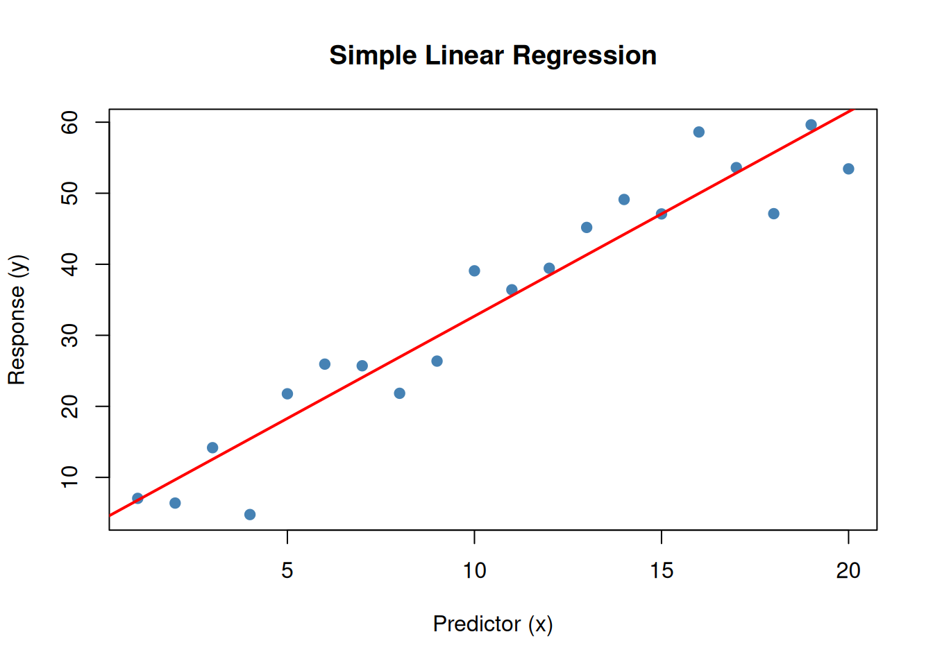
lm(y ~ x)fits the model: \(y = \beta_0 + \beta_1 x + \varepsilon\)- The
~operator means “is modeled as” - We estimate \(\beta_0\) (intercept) and \(\beta_1\) (slope)
- The true value for \(\beta_0\) is 2 and \(\beta_1\) is 3
model1$coefficients(Intercept) x
3.913423 2.878431 Matrix Form
Linear models can be expressed in matrix notation; so instead of:
\[ y = \beta_0 + \beta_1 x_1 + \beta_2 x_2 + ... + \beta_p x_p + \varepsilon \]
we have:
\[\mathbf{y} = \mathbf{X}\boldsymbol{\beta} + \boldsymbol{\varepsilon}\]
Where:
- \(\mathbf{y}\) is an \(n \times 1\) vector of responses (observations)
- \(\mathbf{X}\) is an \(n \times p\) design matrix, also called model matrix
- \(\boldsymbol{\beta}\) is a \(p \times 1\) vector of coefficients
- \(\boldsymbol{\varepsilon}\) is an \(n \times 1\) vector of errors
The design matrix for our simple model.
- Column 1 is all 1’s (for the intercept)
- Column 2 contains our predictor variable
x
set.seed(1984)
x <- sample(x = 1:20)
X <- model.matrix(~ x)
X
(Intercept) x
1 1 8
2 1 17
3 1 14
4 1 15
5 1 20
6 1 1
7 1 13
8 1 4
9 1 16
10 1 19
11 1 18
12 1 6
13 1 7
14 1 5
15 1 12
16 1 2
17 1 9
18 1 10
19 1 11
20 1 3
attr(,"assign")
[1] 0 1The design matrix \(\mathbf{X}\) encodes the structure of our experiment. Each row represents an observation, and each column represents a parameter in the model.
Categorical Variables
Linear models can handle categorical variables.
set.seed(1984)
group <- factor(rep(c("Control", "Treatment"), each = 10))
expression <- c(
  rnorm(10, mean = 5, sd = 1),
  rnorm(10, mean = 8, sd = 1)
)

model2 <- lm(expression ~ group)
summary(model2)
Call:
lm(formula = expression ~ group)

Residuals:
    Min      1Q  Median      3Q     Max
-2.0079 -0.5356  0.1920  0.7560  1.6310

Coefficients:
               Estimate Std. Error t value Pr(>|t|)
(Intercept)      5.1618     0.3361  15.358 8.68e-12 ***
groupTreatment   2.9313     0.4753   6.167 8.02e-06 ***
---
Signif. codes:  0 '***' 0.001 '**' 0.01 '*' 0.05 '.' 0.1 ' ' 1

Residual standard error: 1.063 on 18 degrees of freedom
Multiple R-squared:  0.6788,    Adjusted R-squared:  0.6609
F-statistic: 38.03 on 1 and 18 DF,  p-value: 8.016e-06
Plot.
boxplot(
  expression ~ group,
  col = c("lightblue", "lightcoral"),
  main = "Gene Expression by Group",
  ylab = "Expression Level"
)
points(jitter(as.numeric(group)), expression, pch = 19)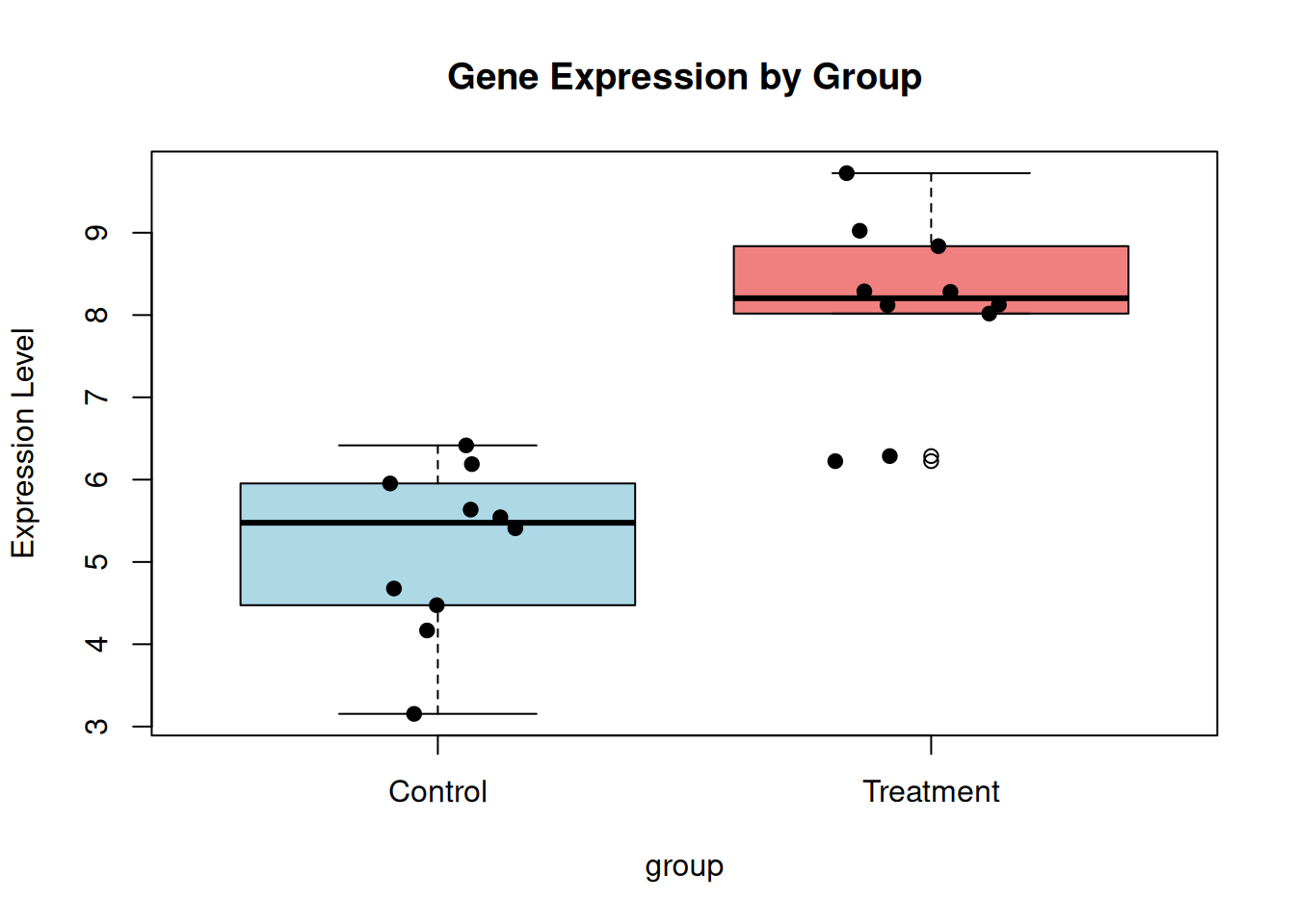
When R encounters a categorical variable, it creates dummy variables and by default, R uses treatment contrasts, where:
- One level is chosen as the reference
- Other levels are compared to the reference
Examine the design matrix:
(Intercept)column (all 1s)groupTreatmentcolumn (0 for reference, 1 for other level)
X2 <- model.matrix(~ group)
print(X2)
(Intercept) groupTreatment
1 1 0
2 1 0
3 1 0
4 1 0
5 1 0
6 1 0
7 1 0
8 1 0
9 1 0
10 1 0
11 1 1
12 1 1
13 1 1
14 1 1
15 1 1
16 1 1
17 1 1
18 1 1
19 1 1
20 1 1
attr(,"assign")
[1] 0 1
attr(,"contrasts")
attr(,"contrasts")$group
[1] "contr.treatment"The model is: \(y_i = \beta_0 + \beta_1 \cdot \text{(Treatment)} + \varepsilon_i\)
Where:
- \(\beta_0\) = mean of Control group
- \(\beta_1\) = difference between Treatment and Control (Treatment - Control)
- When Treatment = 0 (Control): \(y = \beta_0\)
- When Treatment = 1 (Treatment): \(y = \beta_0 + \beta_1\)
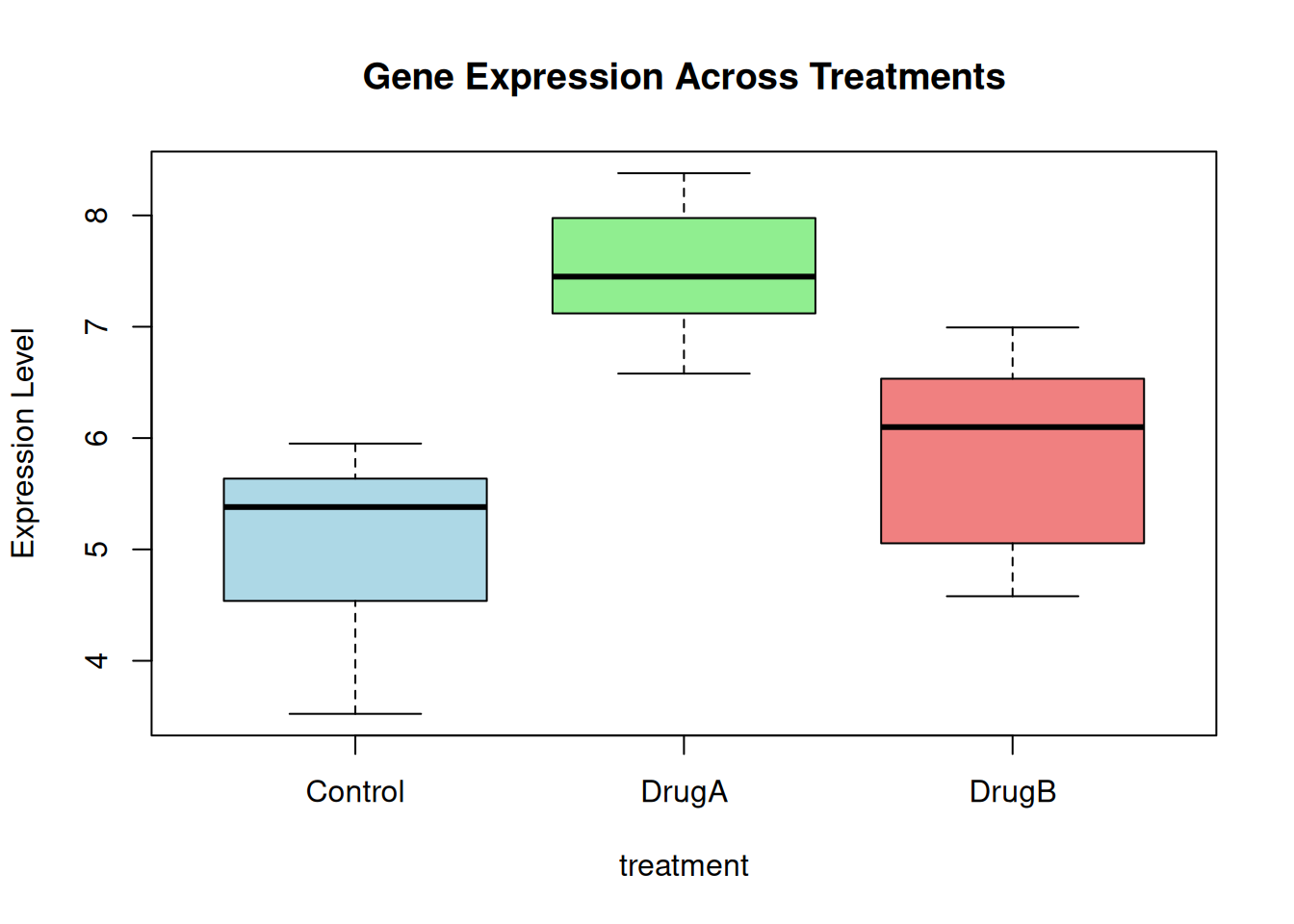
Multiple Groups
Let’s extend to three groups:
set.seed(1984)
treatment <- factor(rep(c("Control", "DrugA", "DrugB"), each = 8))
gene_expr <- c(
  rnorm(8, mean = 5, sd = 0.8),
  rnorm(8, mean = 7, sd = 0.8),
  rnorm(8, mean = 6, sd = 0.8)
)

model3 <- lm(gene_expr ~ treatment)
summary(model3)
Call:
lm(formula = gene_expr ~ treatment)

Residuals:
    Min      1Q  Median      3Q     Max
-1.5497 -0.4135  0.2303  0.5132  1.1252

Coefficients:
               Estimate Std. Error t value Pr(>|t|)
(Intercept)      5.0728     0.2771  18.306 2.18e-14 ***
treatmentDrugA   2.4335     0.3919   6.209 3.69e-06 ***
treatmentDrugB   0.7956     0.3919   2.030   0.0552 .
---
Signif. codes:  0 '***' 0.001 '**' 0.01 '*' 0.05 '.' 0.1 ' ' 1

Residual standard error: 0.7838 on 21 degrees of freedom
Multiple R-squared:  0.6563,    Adjusted R-squared:  0.6236
F-statistic: 20.05 on 2 and 21 DF,  p-value: 1.349e-05
Plot.
boxplot(
  gene_expr ~ treatment, col = c("lightblue", "lightgreen", "lightcoral"),
  main = "Gene Expression Across Treatments",
  ylab = "Expression Level"
)
Model matrix.
X3 <- model.matrix(~ treatment)
print(X3)
(Intercept) treatmentDrugA treatmentDrugB
1 1 0 0
2 1 0 0
3 1 0 0
4 1 0 0
5 1 0 0
6 1 0 0
7 1 0 0
8 1 0 0
9 1 1 0
10 1 1 0
11 1 1 0
12 1 1 0
13 1 1 0
14 1 1 0
15 1 1 0
16 1 1 0
17 1 0 1
18 1 0 1
19 1 0 1
20 1 0 1
21 1 0 1
22 1 0 1
23 1 0 1
24 1 0 1
attr(,"assign")
[1] 0 1 1
attr(,"contrasts")
attr(,"contrasts")$treatment
[1] "contr.treatment"With three groups, the design matrix has:
- 1 intercept column
- 2 dummy variable columns (for DrugA and DrugB)
- Control is the reference level
The model is: \[y_i = \beta_0 + \beta_1 \cdot \text{DrugA}_i + \beta_2 \cdot \text{DrugB}_i + \varepsilon_i\]
Where:
- \(\beta_0\) = mean of Control
- \(\beta_1\) = DrugA - Control
- \(\beta_2\) = DrugB - Control
Design Matrix Summary
The design matrix or model matrix is the bridge between your experimental design and the statistical model. It’s a matrix where:
- Rows = samples/observations
- Columns = parameters in the model (coefficients to estimate)
The design matrix tells the model:
- What groups/conditions each sample belongs to
- What parameters need to be estimated
- How to structure the comparison
Types of Design Matrices
There are two main parameterizations:
- Treatment Contrast (Default in R)
groups <- factor(rep(c("A", "B", "C"), each = 4))

design_treatment <- model.matrix(~groups)
colnames(design_treatment)
[1] "(Intercept)" "groupsB" "groupsC" design_treatment (Intercept) groupsB groupsC
1 1 0 0
2 1 0 0
3 1 0 0
4 1 0 0
5 1 1 0
6 1 1 0
7 1 1 0
8 1 1 0
9 1 0 1
10 1 0 1
11 1 0 1
12 1 0 1
attr(,"assign")
[1] 0 1 1
attr(,"contrasts")
attr(,"contrasts")$groups
[1] "contr.treatment"(Intercept): mean of group A (reference)groupsB: difference B - AgroupsC: difference C - A
Cell means model - design matrix with no intercept, all groups explicit
design_means <- model.matrix(~ 0 + groups)
colnames(design_means)
[1] "groupsA" "groupsB" "groupsC"design_means groupsA groupsB groupsC
1 1 0 0
2 1 0 0
3 1 0 0
4 1 0 0
5 0 1 0
6 0 1 0
7 0 1 0
8 0 1 0
9 0 0 1
10 0 0 1
11 0 0 1
12 0 0 1
attr(,"assign")
[1] 1 1 1
attr(,"contrasts")
attr(,"contrasts")$groups
[1] "contr.treatment"Each coefficient directly represents a group mean; this is useful when you want to make custom comparisons:
groupsA: mean of group AgroupsB: mean of group BgroupsC: mean of group C
Creating Design Matrices
2 genotypes by 2 treatments.
genotype <- factor(rep(c("WT", "Mutant"), each = 6))
treatment <- factor(rep(rep(c("Control", "Treated"), each = 3), 2))

samples <- data.frame(
  Sample = paste0("S", 1:12),
  Genotype = genotype,
  Treatment = treatment
)

samples
Sample Genotype Treatment
1 S1 WT Control
2 S2 WT Control
3 S3 WT Control
4 S4 WT Treated
5 S5 WT Treated
6 S6 WT Treated
7 S7 Mutant Control
8 S8 Mutant Control
9 S9 Mutant Control
10 S10 Mutant Treated
11 S11 Mutant Treated
12 S12 Mutant TreatedDesign matrix with interaction.
design_interaction <- model.matrix(~ Genotype * Treatment, data = samples)
design_interaction
(Intercept) GenotypeWT TreatmentTreated GenotypeWT:TreatmentTreated
1 1 1 0 0
2 1 1 0 0
3 1 1 0 0
4 1 1 1 1
5 1 1 1 1
6 1 1 1 1
7 1 0 0 0
8 1 0 0 0
9 1 0 0 0
10 1 0 1 0
11 1 0 1 0
12 1 0 1 0
attr(,"assign")
[1] 0 1 2 3
attr(,"contrasts")
attr(,"contrasts")$Genotype
[1] "contr.treatment"
attr(,"contrasts")$Treatment
[1] "contr.treatment"The model with interaction:
\[ y = \beta_0 + \beta_1 \cdot \text{Mutant} + \beta_2 \cdot \text{Treated} + \beta_3 \cdot \text{Mutant:Treated} + \varepsilon \]
Where:
- \(\beta_0\) = WT Control mean
- \(\beta_1\) = (Mutant Control) - (WT Control)
- \(\beta_2\) = (WT Treated) - (WT Control)
- \(\beta_3\) = interaction effect (additional effect of treatment in Mutant beyond additive)
Contrast Matrices
A contrast is a linear combination of parameters that represents a specific biological question or comparison of interest.
Mathematically, a contrast is: \(\psi = c_1\beta_1 + c_2\beta_2 + ... + c_p\beta_p\)
Where \(c_1, c_2, ..., c_p\) are the contrast coefficients.
The model parameters might not directly answer your biological question. Contrasts allow you to:
- Test specific hypotheses
- Make comparisons not directly represented in the model
- Test combinations of effects
Simple Contrasts Example
Using the 3 group example, where the coefficients are:
- 0 = Control mean
- 1 = DrugA - Control
- 2 = DrugB - Control
Compare DrugA vs DrugB.
contrast_A_vs_B <- c(0, 1, -1)
names(contrast_A_vs_B) <- c("Intercept", "DrugA", "DrugB")
contrast_A_vs_B
Intercept DrugA DrugB
0 1 -1 Contrast Matrix
When there are multiple contrasts, they are organised into a contrast matrix:
- Rows = parameters in the model
- Columns = different contrasts (comparisons)
If we are interested in DrugA versus DrugB, we need to construct the contrast:
- DrugA vs Control (already in model)
- DrugB vs Control (already in model)
- DrugA vs DrugB (need to construct)
contrast_matrix <- matrix(
  c(
    0,0,0,
    1,0,1,
    0,1,-1
  ),
  nrow = 3,
  ncol = 3,
  byrow = FALSE
)

rownames(contrast_matrix) <- c("Intercept", "DrugA", "DrugB")
colnames(contrast_matrix) <- c("DrugA_vs_Control", "DrugB_vs_Control", "DrugA_vs_DrugB")
contrast_matrix
DrugA_vs_Control DrugB_vs_Control DrugA_vs_DrugB
Intercept 0 1 0
DrugA 0 0 1
DrugB 0 1 -1Making Contrasts with Cell Means Model
Contrasts are often more intuitive with a cell means model (no intercept).
- 1 = mean of A
- 2 = mean of B
- 3 = mean of C
groups_contrast <- matrix(
  c(
    1,1,0,0.5,
    -1,0,1,0.5,
    0,-1,-1,-1
  ),
  nrow = 3,
  ncol = 4,
  byrow = FALSE
)

rownames(groups_contrast) <- c("groupA", "groupB", "groupC")
colnames(groups_contrast) <- c("A_vs_B", "A_vs_C", "B_vs_C", "AvgAB_vs_C")
groups_contrast
A_vs_B A_vs_C B_vs_C AvgAB_vs_C
groupA 1 0.5 1.0 -1
groupB 1 -1.0 0.5 -1
groupC 0 0.0 0.0 -1Contrasts allow you to test any comparison.
Gene Expression Data
Gene expression experiments measure the expression level of thousands of genes across multiple samples. The data structure in R is typically:
- Rows = genes (features)
- Columns = samples (observations)
- Values = expression measurements (counts, intensities, etc.)
A small gene expression dataset.
set.seed(1984)
n_genes <- 8
n_samples <- 12

sample_info <- data.frame(
  Sample = paste0("S", 1:n_samples),
  Genotype = factor(rep(c("WT", "Mutant"), each = 6)),
  Treatment = factor(rep(rep(c("Control", "Treated"), each = 3), 2))
)
sample_info
Sample Genotype Treatment
1 S1 WT Control
2 S2 WT Control
3 S3 WT Control
4 S4 WT Treated
5 S5 WT Treated
6 S6 WT Treated
7 S7 Mutant Control
8 S8 Mutant Control
9 S9 Mutant Control
10 S10 Mutant Treated
11 S11 Mutant Treated
12 S12 Mutant TreatedExpression data.
expr_data <- matrix(
  rnorm(n_genes * n_samples, mean = 7, sd = 0.5),
  nrow = n_genes,
  ncol = n_samples
)

rownames(expr_data) <- paste0("Gene", 1:n_genes)
colnames(expr_data) <- sample_info$Sample

expr_data[1, sample_info$Treatment == "Treated"] <-
  expr_data[1, sample_info$Treatment == "Treated"] + 2

expr_data[2, sample_info$Genotype == "Mutant"] <-
  expr_data[2, sample_info$Genotype == "Mutant"] + 1.5

expr_data[3, sample_info$Genotype == "Mutant" & sample_info$Treatment == "Treated"] <-
  expr_data[3, sample_info$Genotype == "Mutant" & sample_info$Treatment == "Treated"] + 2

round(expr_data, 2)
S1 S2 S3 S4 S5 S6 S7 S8 S9 S10 S11 S12
Gene1 7.20 6.74 7.06 8.99 9.30 9.02 6.67 6.68 7.81 9.15 9.10 10.11
Gene2 6.84 7.71 6.11 7.12 7.48 7.40 9.05 8.09 8.36 8.22 8.78 8.45
Gene3 7.32 7.14 7.06 7.05 7.15 6.95 7.62 6.66 6.73 8.79 8.77 8.96
Gene4 6.08 7.14 6.14 7.41 6.57 6.33 6.68 6.99 6.69 6.87 6.28 6.71
Gene5 7.48 7.42 7.62 6.71 8.25 7.62 6.51 6.63 7.06 7.25 7.08 6.08
Gene6 7.59 7.51 7.21 7.50 6.86 7.59 6.41 7.33 7.45 6.81 7.59 7.58
Gene7 7.27 7.01 6.68 6.45 6.83 6.77 6.81 7.83 6.75 6.62 6.76 7.62
Gene8 6.58 7.86 7.45 6.26 7.12 7.57 6.22 6.83 6.46 6.76 6.56 7.37Many Genes but Few Samples
In typical gene expression experiments:
- Tens of thousands of genes
- Relatively few samples (often < 10 per group)
- Need to fit a separate model for each gene
This creates statistical challenges:
- Multiple testing: Testing thousands of genes inflates false positive rates
- Low power: Few samples means less ability to detect true differences
- Variance estimation: Hard to estimate variance reliably with few samples
The packages limma and edgeR use empirical Bayes methods to borrow information across genes.
Linear Models for Microarray and Omics Data
Linear Models for Microarray and Omics Data (limma) uses linear models to analyse gene expression data. It was originally designed for microarrays but can now be used for different types of omics datasets.
- Fits a linear model to each gene
- Uses empirical Bayes methods to borrow information across genes
- Improves variance estimates (moderated t-statistics)
- Handles complex experimental designs easily
The typical limma workflow:
- Create design matrix - encode experimental design
- Fit linear model - estimate coefficients for each gene
- Define contrasts - specify comparisons of interest
- Apply empirical Bayes - moderate variance estimates
- Test significance - compute p-values and adjusted p-values
Install {limma} if not already.
BiocManager::install("limma")Design Matrix
Create cell means model design matrix.
design <- model.matrix(~ 0 + Genotype + Treatment, data = sample_info)
colnames(design) <- c("WT", "Mutant", "Treated")
design
WT Mutant Treated
1 0 1 0
2 0 1 0
3 0 1 0
4 0 1 1
5 0 1 1
6 0 1 1
7 1 0 0
8 1 0 0
9 1 0 0
10 1 0 1
11 1 0 1
12 1 0 1
attr(,"assign")
[1] 1 1 2
attr(,"contrasts")
attr(,"contrasts")$Genotype
[1] "contr.treatment"
attr(,"contrasts")$Treatment
[1] "contr.treatment"Fit Linear Model to Each Gene
Fit the model to all genes.
fit <- lmFit(expr_data, design)
fit$coefficients[1:4, ]
WT Mutant Treated
Gene1 7.124410 6.926501 2.25463755
Gene2 8.384105 7.002418 0.21553041
Gene3 7.493739 6.682573 0.85548382
Gene4 6.665348 6.576641 0.07290393The lmFit function fits a linear model to each gene
(each row) using the same design matrix.
Define Contrasts
We want to test:
- Treatment effect (Treated vs Control, averaging over genotypes)
- Genotype effect (Mutant vs WT, averaging over treatments)
- Interaction (is treatment effect different in Mutant vs WT?)
makeContrasts() creates a contrast matrix.
contrast_matrix <- makeContrasts(
  TreatmentEffect = Treated,
  GenotypeEffect = Mutant - WT,
  levels = design
)
contrast_matrix
Contrasts
Levels TreatmentEffect GenotypeEffect
WT 0 -1
Mutant 0 1
Treated 1 0Apply contrasts to the fit.
fit2 <- contrasts.fit(fit, contrast_matrix)contrasts.fit computes the contrasts for each gene and
fit2 contains the effect sizes for our comparisons of
interest.
Empirical Bayes Moderation
Apply empirical Bayes moderation using eBayes():
- Estimate a prior distribution for variances across all genes
- Shrink each gene’s variance estimate toward this prior
- This “borrows information” across genes and esults in more stable variance estimates and better power
fit2 <- eBayes(fit2)This is important because:
- With few samples, variance estimates are unreliable
- Some genes might have very small estimated variance just by chance
- This leads to huge (false positive) t-statistics
- Empirical Bayes shrinks extreme variances toward the average
- This reduces false positives while maintaining power
Extract Results
Get results for treatment effect.
results_treatment <- topTable(
  fit2,
  coef = "TreatmentEffect",
  number = Inf,
  sort.by = "P"
)
results_treatment
logFC AveExpr t P.Value adj.P.Val B
Gene1 2.25463755 8.152774 7.9703249 1.741914e-11 1.393531e-10 24.473675
Gene3 0.85548382 7.515898 3.0242040 3.453543e-03 1.381417e-02 -2.519759
Gene7 -0.21567877 6.949564 -0.7624418 4.482870e-01 8.908495e-01 -6.771026
Gene2 0.21553041 7.801027 0.7619173 4.485980e-01 8.908495e-01 -6.771423
Gene4 0.07290393 6.657446 0.2577213 7.973572e-01 8.908495e-01 -7.026612
Gene6 0.06980816 7.286444 0.2467775 8.057827e-01 8.908495e-01 -7.029353
Gene5 0.04478622 7.141997 0.1583229 8.746456e-01 8.908495e-01 -7.047140
Gene8 0.03895690 6.921294 0.1377158 8.908495e-01 8.908495e-01 -7.050168Get results for genotype effect.
results_genotype <- topTable(
  fit2,
  coef = "GenotypeEffect",
  number = Inf,
  sort.by = "P"
)

results_genotype
logFC AveExpr t P.Value adj.P.Val B
Gene2 -1.38168673 7.801027 -4.8843736 6.067869e-06 4.854295e-05 5.128926
Gene3 -0.81116587 7.515898 -2.8675365 5.422740e-03 2.169096e-02 -2.537630
Gene5 0.74801262 7.141997 2.6442847 1.004222e-02 2.677925e-02 -3.141038
Gene8 0.44348055 6.921294 1.5677394 1.213267e-01 2.426534e-01 -5.364573
Gene7 -0.23149404 6.949564 -0.8183500 4.158576e-01 5.893500e-01 -6.241402
Gene1 -0.19790915 8.152774 -0.6996247 4.864160e-01 5.893500e-01 -6.329777
Gene6 0.18478829 7.286444 0.6532415 5.156813e-01 5.893500e-01 -6.360547
Gene4 -0.08870715 6.657446 -0.3135869 7.547415e-01 7.547415e-01 -6.521578The columns
logFC: log2 fold change (effect size from the contrast)AveExpr: average expression level across all samplest: moderated t-statisticP.Value: p-value from moderated t-statisticadj.P.Val: adjusted p-value (controls false discovery rate)B: log-odds of differential expression
limma can also be used for RNA-seq count data with the voom transformation.
Summary
- Linear models represent relationships as: \(y = \mathbf{X}\boldsymbol{\beta} + \boldsymbol{\varepsilon}\)
- Design matrices (\(\mathbf{X}\)) encode experimental structure
- Contrasts specify biological questions as linear combinations of parameters
- limma uses linear models with empirical Bayes for continuous gene expression data
sessionInfo()R version 4.5.0 (2025-04-11)
Platform: x86_64-pc-linux-gnu
Running under: Ubuntu 24.04.3 LTS
Matrix products: default
BLAS: /usr/lib/x86_64-linux-gnu/openblas-pthread/libblas.so.3
LAPACK: /usr/lib/x86_64-linux-gnu/openblas-pthread/libopenblasp-r0.3.26.so; LAPACK version 3.12.0
locale:
[1] LC_CTYPE=en_US.UTF-8 LC_NUMERIC=C
[3] LC_TIME=en_US.UTF-8 LC_COLLATE=en_US.UTF-8
[5] LC_MONETARY=en_US.UTF-8 LC_MESSAGES=en_US.UTF-8
[7] LC_PAPER=en_US.UTF-8 LC_NAME=C
[9] LC_ADDRESS=C LC_TELEPHONE=C
[11] LC_MEASUREMENT=en_US.UTF-8 LC_IDENTIFICATION=C
time zone: Etc/UTC
tzcode source: system (glibc)
attached base packages:
[1] stats graphics grDevices utils datasets methods base
other attached packages:
[1] limma_3.64.3 lubridate_1.9.4 forcats_1.0.0 stringr_1.5.1
[5] dplyr_1.1.4 purrr_1.0.4 readr_2.1.5 tidyr_1.3.1
[9] tibble_3.3.0 ggplot2_3.5.2 tidyverse_2.0.0 workflowr_1.7.1
loaded via a namespace (and not attached):
[1] sass_0.4.10 generics_0.1.4 stringi_1.8.7 hms_1.1.3
[5] digest_0.6.37 magrittr_2.0.3 timechange_0.3.0 evaluate_1.0.3
[9] grid_4.5.0 RColorBrewer_1.1-3 fastmap_1.2.0 rprojroot_2.0.4
[13] jsonlite_2.0.0 processx_3.8.6 whisker_0.4.1 ps_1.9.1
[17] promises_1.3.3 httr_1.4.7 scales_1.4.0 jquerylib_0.1.4
[21] cli_3.6.5 rlang_1.1.6 withr_3.0.2 cachem_1.1.0
[25] yaml_2.3.10 tools_4.5.0 tzdb_0.5.0 httpuv_1.6.16
[29] vctrs_0.6.5 R6_2.6.1 lifecycle_1.0.4 git2r_0.36.2
[33] fs_1.6.6 pkgconfig_2.0.3 callr_3.7.6 pillar_1.10.2
[37] bslib_0.9.0 later_1.4.2 gtable_0.3.6 glue_1.8.0
[41] Rcpp_1.0.14 statmod_1.5.0 xfun_0.52 tidyselect_1.2.1
[45] rstudioapi_0.17.1 knitr_1.50 farver_2.1.2 htmltools_0.5.8.1
[49] rmarkdown_2.29 compiler_4.5.0 getPass_0.2-4