Linear algebra basics
2024-04-21
Last updated: 2024-04-21
Checks: 7 0
Knit directory: muse/
This reproducible R Markdown analysis was created with workflowr (version 1.7.1). The Checks tab describes the reproducibility checks that were applied when the results were created. The Past versions tab lists the development history.
Great! Since the R Markdown file has been committed to the Git repository, you know the exact version of the code that produced these results.
Great job! The global environment was empty. Objects defined in the global environment can affect the analysis in your R Markdown file in unknown ways. For reproduciblity it’s best to always run the code in an empty environment.
The command set.seed(20200712) was run prior to running
the code in the R Markdown file. Setting a seed ensures that any results
that rely on randomness, e.g. subsampling or permutations, are
reproducible.
Great job! Recording the operating system, R version, and package versions is critical for reproducibility.
Nice! There were no cached chunks for this analysis, so you can be confident that you successfully produced the results during this run.
Great job! Using relative paths to the files within your workflowr project makes it easier to run your code on other machines.
Great! You are using Git for version control. Tracking code development and connecting the code version to the results is critical for reproducibility.
The results in this page were generated with repository version 58aaac2. See the Past versions tab to see a history of the changes made to the R Markdown and HTML files.
Note that you need to be careful to ensure that all relevant files for
the analysis have been committed to Git prior to generating the results
(you can use wflow_publish or
wflow_git_commit). workflowr only checks the R Markdown
file, but you know if there are other scripts or data files that it
depends on. Below is the status of the Git repository when the results
were generated:
Ignored files:
    Ignored:    .Rproj.user/
    Ignored:    r_packages_4.3.3/
Note that any generated files, e.g. HTML, png, CSS, etc., are not included in this status report because it is ok for generated content to have uncommitted changes.
These are the previous versions of the repository in which changes were
made to the R Markdown (analysis/linear_algebra.Rmd) and
HTML (docs/linear_algebra.html) files. If you’ve configured
a remote Git repository (see ?wflow_git_remote), click on
the hyperlinks in the table below to view the files as they were in that
past version.
| File | Version | Author | Date | Message |
|---|---|---|---|---|
| Rmd | 58aaac2 | Dave Tang | 2024-04-21 | Paul Dirac’s notation |
| html | c578a55 | Dave Tang | 2024-04-21 | Build site. |
| Rmd | 2442c92 | Dave Tang | 2024-04-21 | Another perpendicular example |
| html | 3d298bc | Dave Tang | 2024-04-21 | Build site. |
| Rmd | ed752d3 | Dave Tang | 2024-04-21 | Orthogonal means perpendicular |
| html | 75b63ae | Dave Tang | 2024-04-20 | Build site. |
| Rmd | fb1ef5b | Dave Tang | 2024-04-20 | Parallelogram law for vector addition |
| html | 8ae3753 | Dave Tang | 2024-04-20 | Build site. |
| Rmd | 97fe3ef | Dave Tang | 2024-04-20 | Fix formula |
| html | 96459ae | Dave Tang | 2024-04-20 | Build site. |
| Rmd | 8d79433 | Dave Tang | 2024-04-20 | Expand and rearrange vectors section |
| html | cd09128 | Dave Tang | 2024-04-20 | Build site. |
| Rmd | 1a7c3c1 | Dave Tang | 2024-04-20 | Linear algebra basics |
Paul Dirac’s notation
How to denote Bra-ket notation in LaTeX?
\[ \langle a | b \rangle \\ \langle p \vert q \rangle \\ \langle a \mid b \rangle \\ \langle \frac{m}{2} \vert \frac{n}{2} \rangle \]
Vectors
A vector is just a list of numbers and the dimension of the vector is the number of numbers in the list. Vectors can be written vertically (column vectors) or horizontally (row vectors). The numbers that make up a vector are often called entries.
A simple five-dimensional (column) vector.
\[ \vec{x} = \begin{pmatrix}8\\6\\7\\5\\3\end{pmatrix} \]
The length of a vector is the distance from its initial point to its terminal point. Calculating vector length is the square root of the sum of squares.
\[ {\lvert}\vec{v}{\rvert} = \sqrt{ \sum_{i=1}^{n}{v_i^2} } \]
Length of the \((3, 1)\) vector.
\[ \sqrt{3^2 + 1^2} = \sqrt{10} \]
A normal vector (or unit vector) is a vector of length 1. For example, the vector \((2/5, 4/5, 1/5, 2/5)\) has length 1.
\[ {\lvert}\vec{u}{\rvert} = \sqrt{(\frac{2}{5})^2 + (\frac{4}{5})^2 + (\frac{1}{5})^2 + (\frac{2}{5})^2} = \sqrt{\frac{4}{25} + \frac{16}{25} + \frac{1}{25} + \frac{4}{25}} = \sqrt{\frac{25}{25}} = 1 \]
We can multiply a vector by a number and in linear algebra, numbers are often called scalars. Scalar multiplication just refers to multiplying by a number. We do this by multiplying each of the entries by the scalar.
\[ \vec{v} = [3, 6, 8, 4] \times 1.5 = [4.5, 9, 12, 6] \]
If we multiply a vector by the reciprocal of its length, we obtain a unit vector. For example the vector \((3, 1)\) has length \(\sqrt{10}\).
\[ \frac{1}{\sqrt{10}} \times \begin{pmatrix}3\\1\end{pmatrix} = \begin{pmatrix} \frac{3}{\sqrt{10}}\\\frac{1}{\sqrt{10}}\end{pmatrix} \\ \sqrt{\bigg(\frac{3}{\sqrt{10}}\bigg)^2 + \bigg(\frac{1}{\sqrt{10}}\bigg)^2} = \sqrt{\frac{9}{10} + \frac{1}{10}} = \sqrt{1} = 1 \]
The dot product or scalar product is an algebraic operation that takes two equal-length sequences of numbers (usually coordinate vectors), and returns a single number. In Euclidean geometry, the dot product of the Cartesian coordinates of two vectors is widely used. It is often called the inner product of Euclidean space, even though it is not the only inner product that can be defined on Euclidean space.
\[ (\vec{x}, \vec{y}) = \vec{x} \cdot \vec{y} = \sum_{i=1}^{n}{x_{i}y_{i}} \]
Given two vectors with the same dimension, we can add them together to get a new vector with the same dimension. The first entry of the new vector is just the addition of the first entries of the two vectors and so on.
\[ A = [a_{1}, a_{2}, \dotsc, a_{n}] \\ B = [b_{1}, b_{2}, \dotsc, b_{n}] \\ A + B = [a_{1} + b_{1}, a_{2} + b_{2}, \dotsc, a_{n} + b_{n}] \]
Vector addition can be pictured by what is often called the parallelogram law for vector addition. If the vector \(B = (1, 2)\) is drawn so that its initial point is at the terminal point of \(A = (3, 1)\), then the vector that goes from the initial point of \(A\) to the terminal point of \(B\) is \(A + B\). This can be drawn giving a triangle.
plot_vec_add <- function(my_df){
  my_df <- rbind(my_df, c(sum(my_df$x), sum(my_df$y)))
  my_arrow <- arrow(length = unit(0.03, "npc"), type = "closed")

  ggplot(my_df, aes(x, y)) +
    geom_point() +
    scale_x_continuous(limits = c(0, max(my_df[, 1]))) +
    scale_y_continuous(limits = c(0, max(my_df[, 2]))) +
    geom_segment(
      aes(
        x=0,
        y=0,
        xend=my_df[1,1],
        yend=my_df[1,2]
      ),
      lty=3,
      arrow = my_arrow
    ) +
    geom_segment(
      aes(
        x=0,
        y=0,
        xend=my_df[2,1],
        yend=my_df[2,2]
      ),
      lty=3,
      arrow = my_arrow
    ) +
    geom_segment(
      aes(
        x=my_df[1,1],
        y=my_df[1,2],
        xend=my_df[3,1],
        yend=my_df[3,2]
      ),
      lty=3,
      arrow = my_arrow
    ) +
    geom_segment(
      aes(
        x=my_df[2,1],
        y=my_df[2,2],
        xend=my_df[3,1],
        yend=my_df[3,2]
      ),
      lty=3,
      arrow = my_arrow
    ) +
    geom_segment(
      aes(
        x=0,
        y=0,
        xend=my_df[3,1],
        yend=my_df[3,2]
      ),
      lty=1,
      arrow = my_arrow
    ) +
    theme_minimal() +
    NULL
}

my_df <- data.frame(
  x = c(3, 1),
  y = c(1, 2)
)

plot_vec_add(my_df)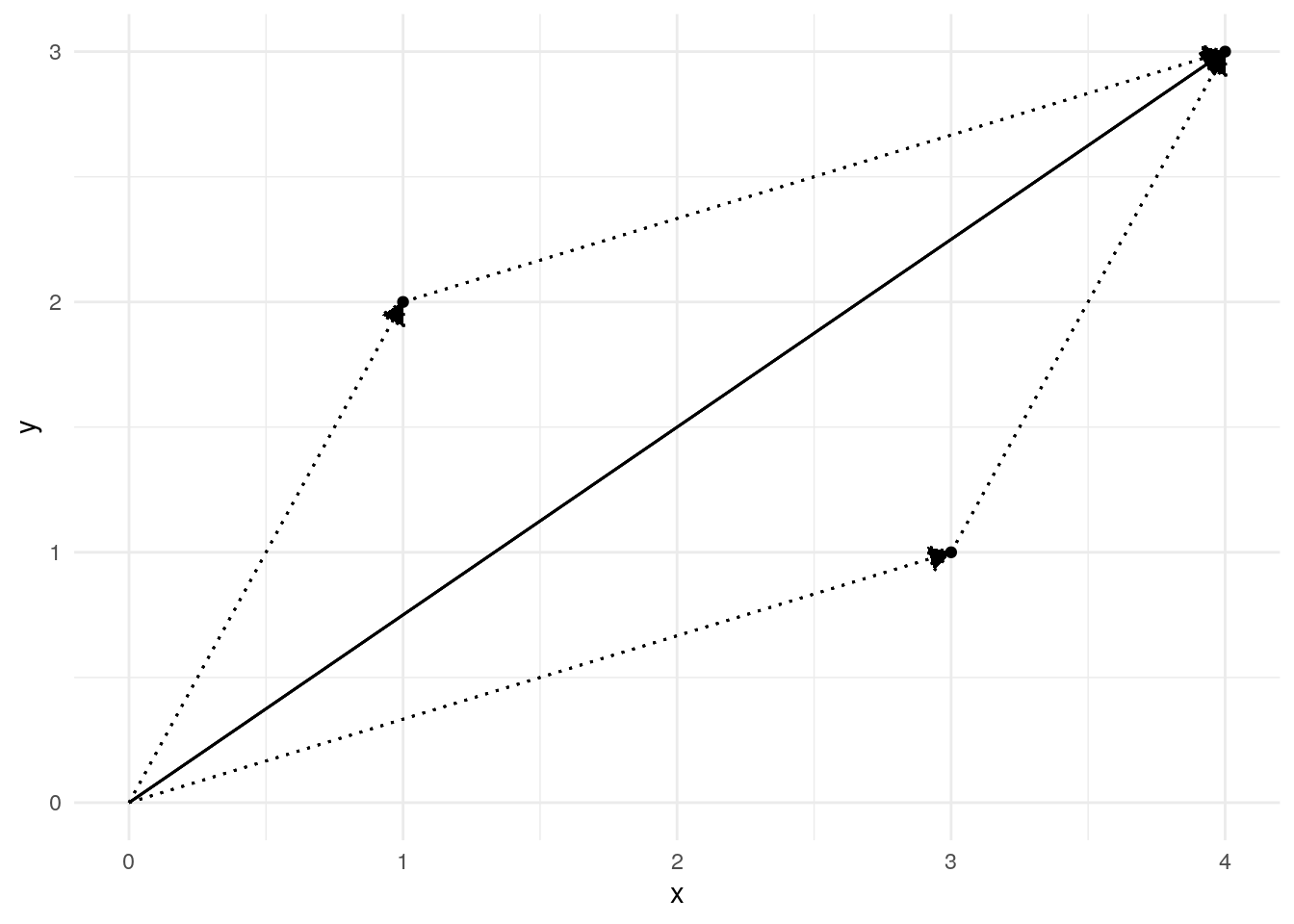
Parallelogram law for vector addition
| Version | Author | Date |
|---|---|---|
| 3d298bc | Dave Tang | 2024-04-21 |
Orthogonality
The parallelogram law for vector addition figure helps us visualise some basic properties of vector addition. One of the most important comes from the Pythagorean theorem. We know that if \(a\), \(b\), and \(c\) represent the lengths of the three sides of a triangle, then \(a^2 + b^2 = c^2\) if and only if the triangle is a right triangle. The figure then tells us that two vectors \(a\) and \(b\) are perpendicular **if and only if and only if \(len(a)^2 + len(b)^2 = len(a+b)^2\).
my_df <- data.frame(
  x = c(0, 4),
  y = c(4, 0)
)
plot_vec_add(my_df)
| Version | Author | Date |
|---|---|---|
| 3d298bc | Dave Tang | 2024-04-21 |
Another example.
my_df <- data.frame(
  x = c(1, 5),
  y = c(5, -1)
)
plot_vec_add(my_df)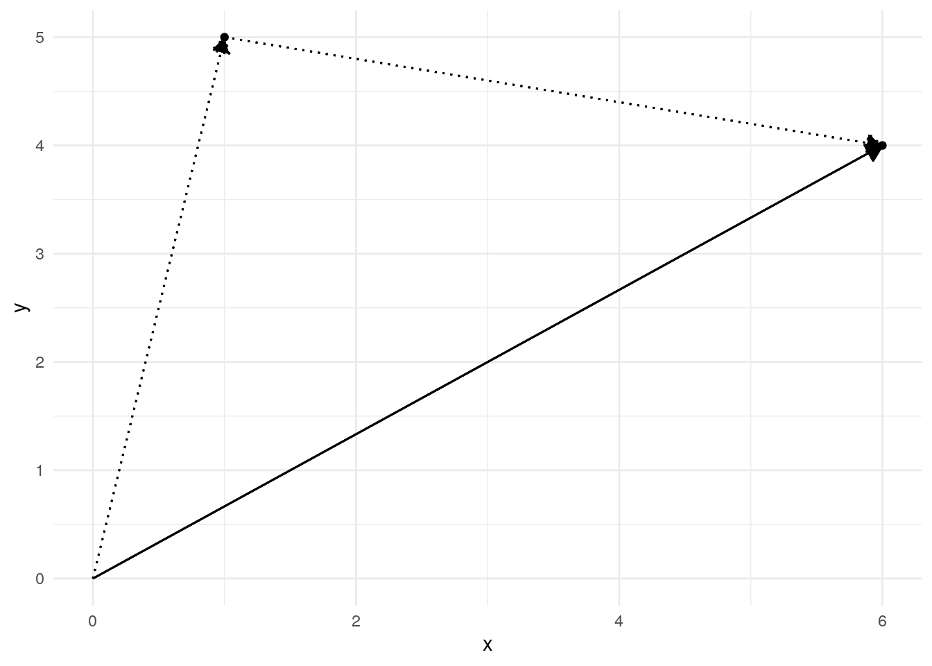
| Version | Author | Date |
|---|---|---|
| c578a55 | Dave Tang | 2024-04-21 |
The word orthogonal means exactly the same thing as perpendicular and it is the word used in linear algebra. Two vectors \(a\) and \(b\) are orthogonal if and only if \(len(a)^2 + len(b)^2 = len(a+b)^2\).
Two vectors are orthogonal if their inner product is zero. Using the example of the plot above where \(a = (1, 5)\) and \(b = (5, -1)\).
\[ [1, 5] \cdot [5, -1] = 1(5) + 5(-1) = 0 \]
Another example.
\[ [2, 1, -2, 4] \cdot [3, -6, 4, 2] = 2(3) + 1(-6) - 2(4) + 4(2) = 0 \]
Vectors of unit length that are orthogonal to each other are said to be orthonormal.
\[ \vec{u} = [2/5, 1/5, -2/5, 4/5] \\ \vec{v} = [3 / \sqrt{65}, -6 / \sqrt{65}, 4 / \sqrt{65}, 2 / \sqrt{65}] \\ {\lvert}\vec{u}\rvert = \sqrt{(2/5)^2 + (1/5)^2 + (-2/5)^2 + (4/5)^2} = 1 \\ {\lvert}\vec{v}\rvert = \sqrt{(3 / \sqrt{65})^2 + (-6 / \sqrt{65})^2 + (4 / \sqrt{65})^2 + (2 / \sqrt{65})^2} = 1 \\ \vec{u} \cdot \vec{v} = \frac{6}{5\sqrt{65}} - \frac{6}{5\sqrt{65}} - \frac{8}{5\sqrt{65}} + \frac{8}{5\sqrt{65}} = 0 \]
If we have row and column vectors with the same dimension, we can multiply them (row on the left and column on the right) to obtain a number.
\[ [a_1, a_2, \cdots, a_n] \begin{bmatrix} b_1 \\ b_2 \\ \vdots \\ b_n \end{bmatrix} = a_1b_1 + a_2b_2 + \cdots + a_nb_n \]
Matrices
Matrix of numbers.
\[ \begin{bmatrix} 17 & 18 & 5 & 5 & 45 & 1 \\ 42 & 28 & 30 & 15 & 115 & 3 \\ 10 & 10 & 10 & 21 & 51 & 2 \\ 28 & 5 & 65 & 39 & 132 & 5 \\ 24 & 26 & 45 & 21 & 116 & 4 \end{bmatrix} \]
Matrix with subscripts and dots
\[ A = \begin{bmatrix} a_{11} & \cdots & a_{1j} & \cdots & a_{1n} \\ \vdots & \ddots & \vdots & \ddots & \vdots \\ a_{i1} & \cdots & a_{ij} & \cdots & a_{in} \\ \vdots & \ddots & \vdots & \ddots & \vdots \\ a_{m1} & \cdots & a_{mj} & \cdots & a_{mn} \end{bmatrix} \]
Square matrix
\[ A = \begin{bmatrix} 1 & 2 & 3 \\ 4 & 5 & 6 \\ 7 & 8 & 9 \end{bmatrix} \]
Transpose.
\[ A = \begin{bmatrix} 1 & 2 & 3 \\ 4 & 5 & 6 \end{bmatrix} \\ A^T = \begin{bmatrix} 1 & 4 \\ 2 & 5 \\ 3 & 6 \end{bmatrix} \]
Matrix multiplication.
\[ AB = \begin{bmatrix} 2 & 1 & 4 \\ 1 & 5 & 2 \end{bmatrix} \begin{bmatrix} 3 & 2 \\ -1 & 4 \\ 1 & 2 \end{bmatrix} = \begin{bmatrix} 9 & 16 \\ 0 & 26 \end{bmatrix} \]
Identity matrix.
\[ AI = \begin{bmatrix}2 & 4 & 6 \\ 1 & 3 & 5 \end{bmatrix} \begin{bmatrix} 1 & 0 & 0 \\ 0 & 1 & 0 \\ 0 & 0 & 1 \end{bmatrix} = \begin{bmatrix}2 & 4 & 6 \\ 1 & 3 & 5 \end{bmatrix} \]
Orthogonal matrix.
\[ AA^T = \begin{bmatrix} 1 & 0 & 0 \\ 0 & 3/5 & -4/5 \\ 0 & 4/5 & 3/5 \end{bmatrix} \begin{bmatrix} 1 & 0 & 0 \\ 0 & 3/5 & 4/5 \\ 0 & -4/5 & 3/5 \end{bmatrix} = \begin{bmatrix} 1 & 0 & 0 \\ 0 & 1 & 0 \\ 0 & 0 & 1 \end{bmatrix} \]
Diagonal matrix
\[ A = \begin{bmatrix} a_{11} & 0 & 0 & 0 \\ 0 & a_{22} & 0 & 0 \\ 0 & 0 & a_{33} & 0 \\ 0 & 0 & 0 & a_{mm} \end{bmatrix} \]
Determinant of a 2x2 matrix.
\[ {\lvert}A\rvert = \left| \begin{array}{cc} a & b \\ c & d \end{array} \right| = ad - bc \]
sessionInfo()R version 4.3.3 (2024-02-29)
Platform: x86_64-pc-linux-gnu (64-bit)
Running under: Ubuntu 22.04.4 LTS
Matrix products: default
BLAS: /usr/lib/x86_64-linux-gnu/openblas-pthread/libblas.so.3
LAPACK: /usr/lib/x86_64-linux-gnu/openblas-pthread/libopenblasp-r0.3.20.so; LAPACK version 3.10.0
locale:
[1] LC_CTYPE=en_US.UTF-8 LC_NUMERIC=C
[3] LC_TIME=en_US.UTF-8 LC_COLLATE=en_US.UTF-8
[5] LC_MONETARY=en_US.UTF-8 LC_MESSAGES=en_US.UTF-8
[7] LC_PAPER=en_US.UTF-8 LC_NAME=C
[9] LC_ADDRESS=C LC_TELEPHONE=C
[11] LC_MEASUREMENT=en_US.UTF-8 LC_IDENTIFICATION=C
time zone: Etc/UTC
tzcode source: system (glibc)
attached base packages:
[1] stats graphics grDevices utils datasets methods base
other attached packages:
[1] lubridate_1.9.3 forcats_1.0.0 stringr_1.5.1 dplyr_1.1.4
[5] purrr_1.0.2 readr_2.1.5 tidyr_1.3.1 tibble_3.2.1
[9] ggplot2_3.5.0 tidyverse_2.0.0 workflowr_1.7.1
loaded via a namespace (and not attached):
[1] sass_0.4.9 utf8_1.2.4 generics_0.1.3 stringi_1.8.3
[5] hms_1.1.3 digest_0.6.35 magrittr_2.0.3 timechange_0.3.0
[9] evaluate_0.23 grid_4.3.3 fastmap_1.1.1 rprojroot_2.0.4
[13] jsonlite_1.8.8 processx_3.8.4 whisker_0.4.1 ps_1.7.6
[17] promises_1.3.0 httr_1.4.7 fansi_1.0.6 scales_1.3.0
[21] jquerylib_0.1.4 cli_3.6.2 rlang_1.1.3 munsell_0.5.1
[25] withr_3.0.0 cachem_1.0.8 yaml_2.3.8 tools_4.3.3
[29] tzdb_0.4.0 colorspace_2.1-0 httpuv_1.6.15 vctrs_0.6.5
[33] R6_2.5.1 lifecycle_1.0.4 git2r_0.33.0 fs_1.6.3
[37] pkgconfig_2.0.3 callr_3.7.6 pillar_1.9.0 bslib_0.7.0
[41] later_1.3.2 gtable_0.3.4 glue_1.7.0 Rcpp_1.0.12
[45] highr_0.10 xfun_0.43 tidyselect_1.2.1 rstudioapi_0.16.0
[49] knitr_1.46 farver_2.1.1 htmltools_0.5.8.1 labeling_0.4.3
[53] rmarkdown_2.26 compiler_4.3.3 getPass_0.2-4