Linear models in R
2026-04-15
Last updated: 2026-04-15
Checks: 7 0
Knit directory: muse/
This reproducible R Markdown analysis was created with workflowr (version 1.7.2). The Checks tab describes the reproducibility checks that were applied when the results were created. The Past versions tab lists the development history.
Great! Since the R Markdown file has been committed to the Git repository, you know the exact version of the code that produced these results.
Great job! The global environment was empty. Objects defined in the global environment can affect the analysis in your R Markdown file in unknown ways. For reproduciblity it’s best to always run the code in an empty environment.
The command set.seed(20200712) was run prior to running
the code in the R Markdown file. Setting a seed ensures that any results
that rely on randomness, e.g. subsampling or permutations, are
reproducible.
Great job! Recording the operating system, R version, and package versions is critical for reproducibility.
Nice! There were no cached chunks for this analysis, so you can be confident that you successfully produced the results during this run.
Great job! Using relative paths to the files within your workflowr project makes it easier to run your code on other machines.
Great! You are using Git for version control. Tracking code development and connecting the code version to the results is critical for reproducibility.
The results in this page were generated with repository version cefef1c. See the Past versions tab to see a history of the changes made to the R Markdown and HTML files.
Note that you need to be careful to ensure that all relevant files for
the analysis have been committed to Git prior to generating the results
(you can use wflow_publish or
wflow_git_commit). workflowr only checks the R Markdown
file, but you know if there are other scripts or data files that it
depends on. Below is the status of the Git repository when the results
were generated:
Ignored files:
    Ignored:    .Rproj.user/
    Ignored:    data/1M_neurons_filtered_gene_bc_matrices_h5.h5
    Ignored:    data/293t/
    Ignored:    data/293t_3t3_filtered_gene_bc_matrices.tar.gz
    Ignored:    data/293t_filtered_gene_bc_matrices.tar.gz
    Ignored:    data/5k_Human_Donor1_PBMC_3p_gem-x_5k_Human_Donor1_PBMC_3p_gem-x_count_sample_filtered_feature_bc_matrix.h5
    Ignored:    data/5k_Human_Donor2_PBMC_3p_gem-x_5k_Human_Donor2_PBMC_3p_gem-x_count_sample_filtered_feature_bc_matrix.h5
    Ignored:    data/5k_Human_Donor3_PBMC_3p_gem-x_5k_Human_Donor3_PBMC_3p_gem-x_count_sample_filtered_feature_bc_matrix.h5
    Ignored:    data/5k_Human_Donor4_PBMC_3p_gem-x_5k_Human_Donor4_PBMC_3p_gem-x_count_sample_filtered_feature_bc_matrix.h5
    Ignored:    data/97516b79-8d08-46a6-b329-5d0a25b0be98.h5ad
    Ignored:    data/Parent_SC3v3_Human_Glioblastoma_filtered_feature_bc_matrix.tar.gz
    Ignored:    data/brain_counts/
    Ignored:    data/cl.obo
    Ignored:    data/cl.owl
    Ignored:    data/jurkat/
    Ignored:    data/jurkat:293t_50:50_filtered_gene_bc_matrices.tar.gz
    Ignored:    data/jurkat_293t/
    Ignored:    data/jurkat_filtered_gene_bc_matrices.tar.gz
    Ignored:    data/pbmc20k/
    Ignored:    data/pbmc20k_seurat/
    Ignored:    data/pbmc3k.csv
    Ignored:    data/pbmc3k.csv.gz
    Ignored:    data/pbmc3k.h5ad
    Ignored:    data/pbmc3k/
    Ignored:    data/pbmc3k_bpcells_mat/
    Ignored:    data/pbmc3k_export.mtx
    Ignored:    data/pbmc3k_matrix.mtx
    Ignored:    data/pbmc3k_seurat.rds
    Ignored:    data/pbmc4k_filtered_gene_bc_matrices.tar.gz
    Ignored:    data/pbmc_1k_v3_filtered_feature_bc_matrix.h5
    Ignored:    data/pbmc_1k_v3_raw_feature_bc_matrix.h5
    Ignored:    data/refdata-gex-GRCh38-2020-A.tar.gz
    Ignored:    data/seurat_1m_neuron.rds
    Ignored:    data/t_3k_filtered_gene_bc_matrices.tar.gz
    Ignored:    r_packages_4.5.2/

Untracked files:
    Untracked:  .claude/
    Untracked:  CLAUDE.md
    Untracked:  analysis/.claude/
    Untracked:  analysis/aucc.Rmd
    Untracked:  analysis/bimodal.Rmd
    Untracked:  analysis/bioc.Rmd
    Untracked:  analysis/bioc_scrnaseq.Rmd
    Untracked:  analysis/chick_weight.Rmd
    Untracked:  analysis/likelihood.Rmd
    Untracked:  analysis/modelling.Rmd
    Untracked:  analysis/sampleqc.Rmd
    Untracked:  analysis/wordpress_readability.Rmd
    Untracked:  bpcells_matrix/
    Untracked:  data/Caenorhabditis_elegans.WBcel235.113.gtf.gz
    Untracked:  data/GCF_043380555.1-RS_2024_12_gene_ontology.gaf.gz
    Untracked:  data/SeuratObj.rds
    Untracked:  data/arab.rds
    Untracked:  data/astronomicalunit.csv
    Untracked:  data/davetang039sblog.WordPress.2026-02-12.xml
    Untracked:  data/femaleMiceWeights.csv
    Untracked:  data/lung_bcell.rds
    Untracked:  m3/
    Untracked:  women.json

Unstaged changes:
    Modified:   analysis/isoform_switch_analyzer.Rmd
Note that any generated files, e.g. HTML, png, CSS, etc., are not included in this status report because it is ok for generated content to have uncommitted changes.
These are the previous versions of the repository in which changes were
made to the R Markdown (analysis/linear_models.Rmd) and
HTML (docs/linear_models.html) files. If you’ve configured
a remote Git repository (see ?wflow_git_remote), click on
the hyperlinks in the table below to view the files as they were in that
past version.
| File | Version | Author | Date | Message |
|---|---|---|---|---|
| Rmd | cefef1c | Dave Tang | 2026-04-15 | Using chick weights |
| html | 00fac99 | Dave Tang | 2025-07-07 | Build site. |
| Rmd | 3c3a848 | Dave Tang | 2025-07-07 | Add source |
| html | 79968d7 | Dave Tang | 2025-07-07 | Build site. |
| Rmd | 3bd2ef6 | Dave Tang | 2025-07-07 | Linear models in practice |
| html | f74eab5 | Dave Tang | 2025-07-07 | Build site. |
| Rmd | fadc325 | Dave Tang | 2025-07-07 | Linear models in R |
From Introduction to Linear Models:
Many of the models we use in data analysis can be presented using matrix algebra. We refer to these types of models as linear models. “Linear” here does not refer to lines, but rather to linear combinations. The representations we describe are convenient because we can write models more succinctly and we have the matrix algebra mathematical machinery to facilitate computation. In this chapter, we will describe in some detail how we use matrix algebra to represent and fit.
In this book, we focus on linear models that represent dichotomous groups: treatment versus control, for example. The effect of diet on mice weights is an example of this type of linear model. Here we describe slightly more complicated models, but continue to focus on dichotomous variables.
As we learn about linear models, we need to remember that we are still working with random variables. This means that the estimates we obtain using linear models are also random variables. Although the mathematics is more complex, the concepts we learned in previous chapters apply here. We begin with some exercises to review the concept of random variables in the context of linear models.
The Design Matrix
From Expressing design formula in R.
Here we will show how to use the two R functions,
formula and model.matrix, in order to produce
design matrices (also known as model matrices) for a
variety of linear models. For example, in the mouse diet examples we
wrote the model as
\[ Y_i = \beta_0 + \beta_1 x_i + \varepsilon_i, i=1,\dots,N \]
with \(Y_i\) the weights and \(x_i\) equal to 1 only when mouse \(i\) receives the high fat diet. We use the term experimental unit to \(N\) different entities from which we obtain a measurement. In this case, the mice are the experimental units.
This is the type of variable we will focus on in this chapter. We call them indicator variables since they simply indicate if the experimental unit had a certain characteristic or not. As we described earlier, we can use linear algebra to represent this model:
\[ \mathbf{Y} = \begin{pmatrix} Y_1\\ Y_2\\ \vdots\\ Y_N \end{pmatrix} , \mathbf{X} = \begin{pmatrix} 1&x_1\\ 1&x_2\\ \vdots\\ 1&x_N \end{pmatrix} , \boldsymbol{\beta} = \begin{pmatrix} \beta_0\\ \beta_1 \end{pmatrix} \mbox{ and } \boldsymbol{\varepsilon} = \begin{pmatrix} \varepsilon_1\\ \varepsilon_2\\ \vdots\\ \varepsilon_N \end{pmatrix} \]
as:
\[ \, \begin{pmatrix} Y_1\\ Y_2\\ \vdots\\ Y_N \end{pmatrix} = \begin{pmatrix} 1&x_1\\ 1&x_2\\ \vdots\\ 1&x_N \end{pmatrix} \begin{pmatrix} \beta_0\\ \beta_1 \end{pmatrix} + \begin{pmatrix} \varepsilon_1\\ \varepsilon_2\\ \vdots\\ \varepsilon_N \end{pmatrix} \]
or simply:
\[ \mathbf{Y}=\mathbf{X}\boldsymbol{\beta}+\boldsymbol{\varepsilon} \]
The design matrix is the matrix \(\mathbf{X}\).
Once we define a design matrix, we are ready to find the least
squares estimates. We refer to this as fitting the model. For
fitting linear models in R, we will directly provide a formula
to the lm function. In this script, we will use the
model.matrix function, which is used internally by the
lm function. This will help us to connect the R
formula with the matrix \(\mathbf{X}\). It will therefore help us
interpret the results from lm.
Choice of design
The choice of design matrix is a critical step in linear modeling since it encodes which coefficients will be fit in the model, as well as the inter-relationship between the samples. A common misunderstanding is that the choice of design follows straightforward from a description of which samples were included in the experiment. This is not the case. The basic information about each sample (whether control or treatment group, experimental batch, etc.) does not imply a single ‘correct’ design matrix. The design matrix additionally encodes various assumptions about how the variables in \(\mathbf{X}\) explain the observed values in \(\mathbf{Y}\), on which the investigator must decide.
For the examples we cover here, we use linear models to make comparisons between different groups. Hence, the design matrices that we ultimately work with will have at least two columns: an intercept column, which consists of a column of 1’s, and a second column, which specifies which samples are in a second group. In this case, two coefficients are fit in the linear model: the intercept, which represents the population average of the first group, and a second coefficient, which represents the difference between the population averages of the second group and the first group. The latter is typically the coefficient we are interested in when we are performing statistical tests: we want to know if there is a difference between the two groups.
We encode this experimental design in R with two pieces. We start
with a formula with the tilde symbol ~. This means that we
want to model the observations using the variables to the right of the
tilde. Then we put the name of a variable, which tells us which samples
are in which group.
Let’s try an example. Suppose we have two groups, control and high
fat diet, with two samples each. For illustrative purposes, we will code
these with 1 and 2 respectively. We should first tell R that these
values should not be interpreted numerically, but as different levels of
a factor. We can then use the paradigm ~ group to,
say, model on the variable group.
group <- factor( c(1,1,2,2) )
model.matrix(~ group)
(Intercept) group2
1 1 0
2 1 0
3 1 1
4 1 1
attr(,"assign")
[1] 0 1
attr(,"contrasts")
attr(,"contrasts")$group
[1] "contr.treatment"(Don’t worry about the attr lines printed beneath the
matrix. We won’t be using this information.)
What about the formula function? We don’t have to
include this. By starting an expression with ~, it is
equivalent to telling R that the expression is a formula:
model.matrix(formula(~ group)) (Intercept) group2
1 1 0
2 1 0
3 1 1
4 1 1
attr(,"assign")
[1] 0 1
attr(,"contrasts")
attr(,"contrasts")$group
[1] "contr.treatment"What happens if we don’t tell R that group should be
interpreted as a factor?
group <- c(1,1,2,2)
model.matrix(~ group)
(Intercept) group
1 1 1
2 1 1
3 1 2
4 1 2
attr(,"assign")
[1] 0 1This is not the design matrix we wanted, and the
reason is that we provided a numeric variable as opposed to an
indicator to the formula and
model.matrix functions, without saying that these numbers
actually referred to different groups. We want the second column to have
only 0 and 1, indicating group membership.
A note about factors: the names of the levels are irrelevant to
model.matrix and lm. All that matters is the
order. For example:
group <- factor(c("control","control","highfat","highfat"))
model.matrix(~ group)
(Intercept) grouphighfat
1 1 0
2 1 0
3 1 1
4 1 1
attr(,"assign")
[1] 0 1
attr(,"contrasts")
attr(,"contrasts")$group
[1] "contr.treatment"produces the same design matrix as our first code chunk.
More groups
Using the same formula, we can accommodate modeling more groups. Suppose we have a third diet:
group <- factor(c(1,1,2,2,3,3))
model.matrix(~ group)
(Intercept) group2 group3
1 1 0 0
2 1 0 0
3 1 1 0
4 1 1 0
5 1 0 1
6 1 0 1
attr(,"assign")
[1] 0 1 1
attr(,"contrasts")
attr(,"contrasts")$group
[1] "contr.treatment"Now we have a third column which specifies which samples belong to the third group.
An alternate formulation of design matrix is possible by specifying
+ 0 in the formula:
group <- factor(c(1,1,2,2,3,3))
model.matrix(~ group + 0)
group1 group2 group3
1 1 0 0
2 1 0 0
3 0 1 0
4 0 1 0
5 0 0 1
6 0 0 1
attr(,"assign")
[1] 1 1 1
attr(,"contrasts")
attr(,"contrasts")$group
[1] "contr.treatment"This group now fits a separate coefficient for each group. We will explore this design in more depth later on.
More variables
We have been using a simple case with just one variable (diet) as an example. In the life sciences, it is quite common to perform experiments with more than one variable. For example, we may be interested in the effect of diet and the difference in sexes. In this case, we have four possible groups:
diet <- factor(c(1,1,1,1,2,2,2,2))
sex <- factor(c("f","f","m","m","f","f","m","m"))
table(diet,sex)
sex
diet f m
1 2 2
2 2 2If we assume that the diet effect is the same for males and females (this is an assumption), then our linear model is:
\[ Y_{i}= \beta_0 + \beta_1 x_{i,1} + \beta_2 x_{i,2} + \varepsilon_i \]
To fit this model in R, we can simply add the additional variable
with a + sign in order to build a design matrix which fits
based on the information in additional variables:
diet <- factor(c(1,1,1,1,2,2,2,2))
sex <- factor(c("f","f","m","m","f","f","m","m"))
model.matrix(~ diet + sex)
(Intercept) diet2 sexm
1 1 0 0
2 1 0 0
3 1 0 1
4 1 0 1
5 1 1 0
6 1 1 0
7 1 1 1
8 1 1 1
attr(,"assign")
[1] 0 1 2
attr(,"contrasts")
attr(,"contrasts")$diet
[1] "contr.treatment"
attr(,"contrasts")$sex
[1] "contr.treatment"The design matrix includes an intercept, a term for diet
and a term for sex. We would say that this linear model
accounts for differences in both the group and condition variables.
However, as mentioned above, the model assumes that the diet effect is
the same for both males and females. We say these are an
additive effect. For each variable, we add an effect regardless
of what the other is. Another model is possible here, which fits an
additional term and which encodes the potential interaction of group and
condition variables. We will cover interaction terms in depth in a later
script.
The interaction model can be written in either of the following two formulas:
model.matrix(~ diet + sex + diet:sex)or
model.matrix(~ diet*sex) (Intercept) diet2 sexm diet2:sexm
1 1 0 0 0
2 1 0 0 0
3 1 0 1 0
4 1 0 1 0
5 1 1 0 0
6 1 1 0 0
7 1 1 1 1
8 1 1 1 1
attr(,"assign")
[1] 0 1 2 3
attr(,"contrasts")
attr(,"contrasts")$diet
[1] "contr.treatment"
attr(,"contrasts")$sex
[1] "contr.treatment"Releveling
The level which is chosen for the reference level is the
level which is contrasted against. By default, this is simply the first
level alphabetically. We can specify that we want group 2 to be the
reference level by either using the relevel function:
group <- factor(c(1,1,2,2))
group <- relevel(group, "2")
model.matrix(~ group)
(Intercept) group1
1 1 1
2 1 1
3 1 0
4 1 0
attr(,"assign")
[1] 0 1
attr(,"contrasts")
attr(,"contrasts")$group
[1] "contr.treatment"or by providing the levels explicitly in the factor
call:
group <- factor(group, levels=c("1","2"))
model.matrix(~ group)
(Intercept) group2
1 1 0
2 1 0
3 1 1
4 1 1
attr(,"assign")
[1] 0 1
attr(,"contrasts")
attr(,"contrasts")$group
[1] "contr.treatment"Where does model.matrix look for the data?
The model.matrix function will grab the variable from
the R global environment, unless the data is explicitly provided as a
data frame to the data argument:
group <- 1:4
model.matrix(~ group, data=data.frame(group=5:8))
(Intercept) group
1 1 5
2 1 6
3 1 7
4 1 8
attr(,"assign")
[1] 0 1Note how the R global environment variable group is
ignored.
Continuous variables
In this chapter, we focus on models based on indicator values. In certain designs, however, we will be interested in using numeric variables in the design formula, as opposed to converting them to factors first. For example, in the falling object example, time was a continuous variable in the model and time squared was also included:
tt <- seq(0,3.4,len=4)
model.matrix(~ tt + I(tt^2))
(Intercept) tt I(tt^2)
1 1 0.000000 0.000000
2 1 1.133333 1.284444
3 1 2.266667 5.137778
4 1 3.400000 11.560000
attr(,"assign")
[1] 0 1 2The I function above is necessary to specify a
mathematical transformation of a variable. For more details, see the
manual page for the I function by typing
?I.
In the life sciences, we could be interested in testing various dosages of a treatment, where we expect a specific relationship between a measured quantity and the dosage, e.g. 0 mg, 10 mg, 20 mg.
The assumptions imposed by including continuous data as variables are typically hard to defend and motivate than the indicator function variables. Whereas the indicator variables simply assume a different mean between two groups, continuous variables assume a very specific relationship between the outcome and predictor variables.
In cases like the falling object, we have the theory of gravitation supporting the model. In the father-son height example, because the data is bivariate normal, it follows that there is a linear relationship if we condition. However, we find that continuous variables are included in linear models without justification to “adjust” for variables such as age. We highly discourage this practice unless the data support the model being used.
Linear models in practice
From Linear models in practice.
The mouse diet example
We will demonstrate how to analyze the high fat diet data using linear models instead of directly applying a t-test. We will demonstrate how ultimately these two approaches are equivalent.
We start by reading in the data and creating a quick stripchart:
dat <- read.csv(filename)
stripchart(dat$Bodyweight ~ dat$Diet, vertical=TRUE, method="jitter",
           main="Bodyweight over Diet")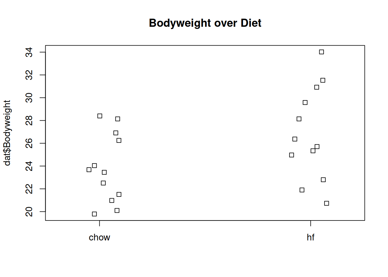
Mice bodyweights stratified by diet.
| Version | Author | Date |
|---|---|---|
| 79968d7 | Dave Tang | 2025-07-07 |
We can see that the high fat diet group appears to have higher weights on average, although there is overlap between the two samples.
For demonstration purposes, we will build the design matrix \(\mathbf{X}\) using the formula
~ Diet. The group with the 1’s in the second column is
determined by the level of Diet which comes second; that
is, the non-reference level.
dat$Diet <- factor(dat$Diet)
levels(dat$Diet)
[1] "chow" "hf" X <- model.matrix(~ Diet, data=dat)
X (Intercept) Diethf
1 1 0
2 1 0
3 1 0
4 1 0
5 1 0
6 1 0
7 1 0
8 1 0
9 1 0
10 1 0
11 1 0
12 1 0
13 1 1
14 1 1
15 1 1
16 1 1
17 1 1
18 1 1
19 1 1
20 1 1
21 1 1
22 1 1
23 1 1
24 1 1
attr(,"assign")
[1] 0 1
attr(,"contrasts")
attr(,"contrasts")$Diet
[1] "contr.treatment"The Mathematics Behind lm()
Before we use our shortcut for running linear models,
lm, we want to review what will happen internally. Inside
of lm, we will form the design matrix \(\mathbf{X}\) and calculate the \(\boldsymbol{\beta}\), which minimizes the
sum of squares using the previously described formula. The formula for
this solution is:
\[ \hat{\boldsymbol{\beta}} = (\mathbf{X}^\top \mathbf{X})^{-1} \mathbf{X}^\top \mathbf{Y} \]
We can calculate this in R using our matrix multiplication operator
%*%, the inverse function solve (Solve a
System of Equations), and the transpose function t.
Y <- dat$Bodyweight
X <- model.matrix(~ Diet, data=dat)
solve(t(X) %*% X) %*% t(X) %*% Y
[,1]
(Intercept) 23.813333
Diethf 3.020833These coefficients are the average of the control group and the difference of the averages:
s <- split(dat$Bodyweight, dat$Diet)
mean(s[["chow"]])
[1] 23.81333mean(s[["hf"]]) - mean(s[["chow"]])[1] 3.020833Finally, we use our shortcut, lm, to run the linear
model:
fit <- lm(Bodyweight ~ Diet, data=dat)
summary(fit)
Call:
lm(formula = Bodyweight ~ Diet, data = dat)

Residuals:
    Min      1Q  Median      3Q     Max
-6.1042 -2.4358 -0.4138  2.8335  7.1858

Coefficients:
            Estimate Std. Error t value Pr(>|t|)
(Intercept)   23.813      1.039  22.912   <2e-16 ***
Diethf         3.021      1.470   2.055   0.0519 .
---
Signif. codes:  0 '***' 0.001 '**' 0.01 '*' 0.05 '.' 0.1 ' ' 1

Residual standard error: 3.6 on 22 degrees of freedom
Multiple R-squared:  0.1611,    Adjusted R-squared:  0.1229
F-statistic: 4.224 on 1 and 22 DF,  p-value: 0.05192
(coefs <- coef(fit))(Intercept) Diethf
23.813333 3.020833 Examining the coefficients
The following plot provides a visualization of the meaning of the coefficients with colored arrows:
stripchart(dat$Bodyweight ~ dat$Diet, vertical=TRUE, method="jitter",
           main="Bodyweight over Diet", ylim=c(0,40), xlim=c(0,3))
a <- -0.25
lgth <- .1
library(RColorBrewer)
cols <- brewer.pal(3,"Dark2")
abline(h=0)
arrows(1+a,0,1+a,coefs[1],lwd=3,col=cols[1],length=lgth)
abline(h=coefs[1],col=cols[1])
arrows(2+a,coefs[1],2+a,coefs[1]+coefs[2],lwd=3,col=cols[2],length=lgth)
abline(h=coefs[1]+coefs[2],col=cols[2])
legend("right",names(coefs),fill=cols,cex=.75,bg="white")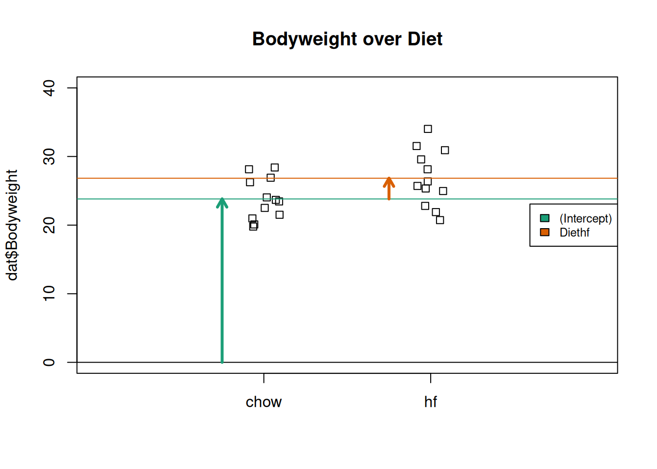
Estimated linear model coefficients for bodyweight data illustrated with arrows.
| Version | Author | Date |
|---|---|---|
| 79968d7 | Dave Tang | 2025-07-07 |
To make a connection with material presented earlier, this simple linear model is actually giving us the same result (the t-statistic and p-value) for the difference as a specific kind of t-test. This is the t-test between two groups with the assumption that the population standard deviation is the same for both groups. This was encoded into our linear model when we assumed that the errors \(\boldsymbol{\varepsilon}\) were all equally distributed.
Although in this case the linear model is equivalent to a t-test, we will soon explore more complicated designs, where the linear model is a useful extension. Below we demonstrate that one does in fact get the exact same results:
Our lm estimates were:
summary(fit)$coefficients Estimate Std. Error t value Pr(>|t|)
(Intercept) 23.813333 1.039353 22.911684 7.642256e-17
Diethf 3.020833 1.469867 2.055174 5.192480e-02And the t-statistic is the same:
ttest <- t.test(s[["hf"]], s[["chow"]], var.equal=TRUE)
summary(fit)$coefficients[2,3]
[1] 2.055174ttest$statistic t
2.055174 Chick weight
The built-in ChickWeight dataset records the body weight
of chicks fed one of four experimental diets, measured every couple of
days from hatching. It is a convenient playground for illustrating the
core concepts of linear modelling: a continuous predictor
(Time), a categorical predictor (Diet), and
repeated measurements on individual chicks (Chick).
head(ChickWeight) weight Time Chick Diet
1 42 0 1 1
2 51 2 1 1
3 59 4 1 1
4 64 6 1 1
5 76 8 1 1
6 93 10 1 1str(ChickWeight)Classes 'nfnGroupedData', 'nfGroupedData', 'groupedData' and 'data.frame': 578 obs. of 4 variables:
$ weight: num 42 51 59 64 76 93 106 125 149 171 ...
$ Time : num 0 2 4 6 8 10 12 14 16 18 ...
$ Chick : Ord.factor w/ 50 levels "18"<"16"<"15"<..: 15 15 15 15 15 15 15 15 15 15 ...
$ Diet : Factor w/ 4 levels "1","2","3","4": 1 1 1 1 1 1 1 1 1 1 ...
- attr(*, "formula")=Class 'formula' language weight ~ Time | Chick
.. ..- attr(*, ".Environment")=<environment: R_EmptyEnv>
- attr(*, "outer")=Class 'formula' language ~Diet
.. ..- attr(*, ".Environment")=<environment: R_EmptyEnv>
- attr(*, "labels")=List of 2
..$ x: chr "Time"
..$ y: chr "Body weight"
- attr(*, "units")=List of 2
..$ x: chr "(days)"
..$ y: chr "(gm)"Growth trajectories vary between chicks and between diets:
ggplot(ChickWeight, aes(x = Time, y = weight, group = Chick, colour = Diet)) +
  geom_line(alpha = 0.6) +
  facet_wrap(~ Diet) +
  theme_bw() +
  labs(x = "Days since hatching", y = "Weight (g)")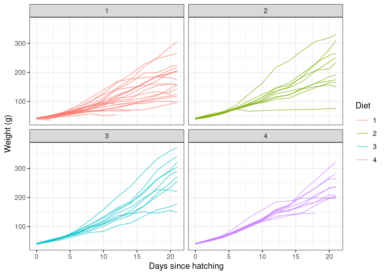
Individual chick growth trajectories, faceted by diet.
A simple linear model
We start with the simplest possible model: weight as a linear function of time, ignoring diet.
\[ \text{weight}_i = \beta_0 + \beta_1\,\text{Time}_i + \varepsilon_i \]
fit_time <- lm(weight ~ Time, data = ChickWeight)
summary(fit_time)
Call:
lm(formula = weight ~ Time, data = ChickWeight)

Residuals:
     Min       1Q   Median       3Q      Max
-138.331  -14.536    0.926   13.533  160.669

Coefficients:
            Estimate Std. Error t value Pr(>|t|)
(Intercept)  27.4674     3.0365   9.046   <2e-16 ***
Time          8.8030     0.2397  36.725   <2e-16 ***
---
Signif. codes:  0 '***' 0.001 '**' 0.01 '*' 0.05 '.' 0.1 ' ' 1

Residual standard error: 38.91 on 576 degrees of freedom
Multiple R-squared:  0.7007,    Adjusted R-squared:  0.7002
F-statistic:  1349 on 1 and 576 DF,  p-value: < 2.2e-16
The two coefficients have a direct, intuitive interpretation:
(Intercept)is the expected weight atTime = 0(the day of hatching).Timeis the average daily weight gain in grams, pooled across all diets and chicks.
ggplot(ChickWeight, aes(x = Time, y = weight)) +
  geom_point(alpha = 0.3) +
  geom_smooth(method = "lm", se = FALSE, colour = "red") +
  theme_bw() +
  labs(x = "Days since hatching", y = "Weight (g)")
`geom_smooth()` using formula = 'y ~ x'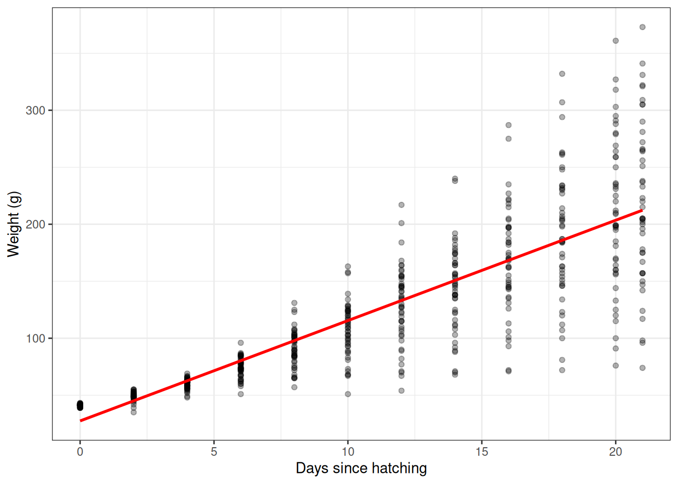
Simple linear regression of weight on time.
Adding a categorical predictor
Pooling across diets hides the effect we probably care about. We add
Diet as an additional predictor. Because Diet
is a factor with four levels, R expands it into three indicator
variables, leaving Diet 1 as the reference level:
\[ \text{weight}_i = \beta_0 + \beta_1\,\text{Time}_i + \beta_2 D2_i + \beta_3 D3_i + \beta_4 D4_i + \varepsilon_i \]
fit_add <- lm(weight ~ Time + Diet, data = ChickWeight)
summary(fit_add)
Call:
lm(formula = weight ~ Time + Diet, data = ChickWeight)

Residuals:
     Min       1Q   Median       3Q      Max
-136.851  -17.151   -2.595   15.033  141.816

Coefficients:
            Estimate Std. Error t value Pr(>|t|)
(Intercept)  10.9244     3.3607   3.251  0.00122 **
Time          8.7505     0.2218  39.451  < 2e-16 ***
Diet2        16.1661     4.0858   3.957 8.56e-05 ***
Diet3        36.4994     4.0858   8.933  < 2e-16 ***
Diet4        30.2335     4.1075   7.361 6.39e-13 ***
---
Signif. codes:  0 '***' 0.001 '**' 0.01 '*' 0.05 '.' 0.1 ' ' 1

Residual standard error: 35.99 on 573 degrees of freedom
Multiple R-squared:  0.7453,    Adjusted R-squared:  0.7435
F-statistic: 419.2 on 4 and 573 DF,  p-value: < 2.2e-16
This is an additive model: every diet is assumed to share
the same growth rate (the single Time coefficient), but
each diet is allowed its own intercept. The Diet2,
Diet3, Diet4 coefficients are the average
difference in weight relative to Diet 1.
Inspecting the design matrix makes the encoding explicit:
head(model.matrix(fit_add)) (Intercept) Time Diet2 Diet3 Diet4
1 1 0 0 0 0
2 1 2 0 0 0
3 1 4 0 0 0
4 1 6 0 0 0
5 1 8 0 0 0
6 1 10 0 0 0Interaction: does diet change the growth rate?
Looking at the trajectory plot, the slopes look different between
diets — chicks on Diet 3 seem to grow faster than those on Diet 1. To
test this we include an interaction between Time and
Diet:
\[ \text{weight}_i = \beta_0 + \beta_1\,\text{Time}_i + \sum_{d=2}^{4} \beta_d D_{d,i} + \sum_{d=2}^{4} \gamma_d\,(D_{d,i}\!\times\!\text{Time}_i) + \varepsilon_i \]
fit_int <- lm(weight ~ Time * Diet, data = ChickWeight)
summary(fit_int)
Call:
lm(formula = weight ~ Time * Diet, data = ChickWeight)

Residuals:
     Min       1Q   Median       3Q      Max
-135.425  -13.757   -1.311   11.069  130.391

Coefficients:
            Estimate Std. Error t value Pr(>|t|)
(Intercept)  30.9310     4.2468   7.283 1.09e-12 ***
Time          6.8418     0.3408  20.076  < 2e-16 ***
Diet2        -2.2974     7.2672  -0.316  0.75202
Diet3       -12.6807     7.2672  -1.745  0.08154 .
Diet4        -0.1389     7.2865  -0.019  0.98480
Time:Diet2    1.7673     0.5717   3.092  0.00209 **
Time:Diet3    4.5811     0.5717   8.014 6.33e-15 ***
Time:Diet4    2.8726     0.5781   4.969 8.92e-07 ***
---
Signif. codes:  0 '***' 0.001 '**' 0.01 '*' 0.05 '.' 0.1 ' ' 1

Residual standard error: 34.07 on 570 degrees of freedom
Multiple R-squared:  0.773, Adjusted R-squared:  0.7702
F-statistic: 277.3 on 7 and 570 DF,  p-value: < 2.2e-16
Now each diet has its own intercept and its own slope. The
Time:Diet2, Time:Diet3 and
Time:Diet4 coefficients are the differences in growth rate
relative to Diet 1. A significant interaction coefficient indicates that
chicks on that diet gain weight at a different rate to those on Diet
1.
ggplot(ChickWeight, aes(x = Time, y = weight, colour = Diet)) +
  geom_point(alpha = 0.3) +
  geom_smooth(method = "lm", se = FALSE) +
  theme_bw() +
  labs(x = "Days since hatching", y = "Weight (g)")
`geom_smooth()` using formula = 'y ~ x'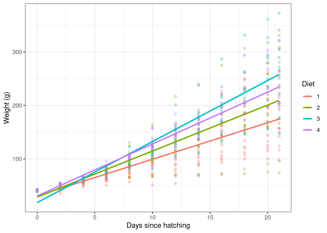
Linear model with a Time-by-Diet interaction: each diet has its own slope and intercept.
Comparing nested models
Each model is a special case of the next. We can compare them
formally with anova(), which performs a sequential
F-test:
anova(fit_time, fit_add, fit_int)Analysis of Variance Table
Model 1: weight ~ Time
Model 2: weight ~ Time + Diet
Model 3: weight ~ Time * Diet
Res.Df RSS Df Sum of Sq F Pr(>F)
1 576 872212
2 573 742336 3 129876 37.302 < 2.2e-16 ***
3 570 661532 3 80804 23.208 3.474e-14 ***
---
Signif. codes: 0 '***' 0.001 '**' 0.01 '*' 0.05 '.' 0.1 ' ' 1Small p-values indicate that the extra parameters significantly
improve the fit. Here, both adding Diet and adding the
Time:Diet interaction are justified by the data.
Extracting the design matrix
For diagnostic work (or when implementing the normal equations by
hand, as we did earlier) it is useful to have the design matrix \(\mathbf{X}\) attached to the fitted model.
Passing x = TRUE to lm stores it in the
returned object:
fit <- lm(weight ~ Diet + Chick, data = ChickWeight, x = TRUE)

design <- model.matrix(fit)
identical(design, fit$x)
[1] TRUEThe design matrix is the bridge between the formula we write and the
matrix algebra lm uses under the hood. Once you are
comfortable reading it, the meaning of every coefficient in the summary
output becomes transparent.
sessionInfo()R version 4.5.2 (2025-10-31)
Platform: x86_64-pc-linux-gnu
Running under: Ubuntu 24.04.4 LTS
Matrix products: default
BLAS: /usr/lib/x86_64-linux-gnu/openblas-pthread/libblas.so.3
LAPACK: /usr/lib/x86_64-linux-gnu/openblas-pthread/libopenblasp-r0.3.26.so; LAPACK version 3.12.0
locale:
[1] LC_CTYPE=en_US.UTF-8 LC_NUMERIC=C
[3] LC_TIME=en_US.UTF-8 LC_COLLATE=en_US.UTF-8
[5] LC_MONETARY=en_US.UTF-8 LC_MESSAGES=en_US.UTF-8
[7] LC_PAPER=en_US.UTF-8 LC_NAME=C
[9] LC_ADDRESS=C LC_TELEPHONE=C
[11] LC_MEASUREMENT=en_US.UTF-8 LC_IDENTIFICATION=C
time zone: Etc/UTC
tzcode source: system (glibc)
attached base packages:
[1] stats graphics grDevices utils datasets methods base
other attached packages:
[1] RColorBrewer_1.1-3 lubridate_1.9.5 forcats_1.0.1 stringr_1.6.0
[5] dplyr_1.2.0 purrr_1.2.1 readr_2.2.0 tidyr_1.3.2
[9] tibble_3.3.1 ggplot2_4.0.2 tidyverse_2.0.0 workflowr_1.7.2
loaded via a namespace (and not attached):
[1] sass_0.4.10 generics_0.1.4 lattice_0.22-7 stringi_1.8.7
[5] hms_1.1.4 digest_0.6.39 magrittr_2.0.4 timechange_0.4.0
[9] evaluate_1.0.5 grid_4.5.2 fastmap_1.2.0 Matrix_1.7-4
[13] rprojroot_2.1.1 jsonlite_2.0.0 processx_3.8.6 whisker_0.4.1
[17] ps_1.9.1 promises_1.5.0 mgcv_1.9-3 httr_1.4.8
[21] scales_1.4.0 jquerylib_0.1.4 cli_3.6.5 rlang_1.1.7
[25] splines_4.5.2 withr_3.0.2 cachem_1.1.0 yaml_2.3.12
[29] otel_0.2.0 tools_4.5.2 tzdb_0.5.0 httpuv_1.6.17
[33] vctrs_0.7.2 R6_2.6.1 lifecycle_1.0.5 git2r_0.36.2
[37] fs_2.0.1 pkgconfig_2.0.3 callr_3.7.6 pillar_1.11.1
[41] bslib_0.10.0 later_1.4.8 gtable_0.3.6 glue_1.8.0
[45] Rcpp_1.1.1 xfun_0.57 tidyselect_1.2.1 rstudioapi_0.18.0
[49] knitr_1.51 farver_2.1.2 nlme_3.1-168 htmltools_0.5.9
[53] labeling_0.4.3 rmarkdown_2.31 compiler_4.5.2 getPass_0.2-4
[57] S7_0.2.1