Differential abundance testing with Milo
2025-01-11
Last updated: 2025-01-11
Checks: 7 0
Knit directory: muse/
This reproducible R Markdown analysis was created with workflowr (version 1.7.1). The Checks tab describes the reproducibility checks that were applied when the results were created. The Past versions tab lists the development history.
Great! Since the R Markdown file has been committed to the Git repository, you know the exact version of the code that produced these results.
Great job! The global environment was empty. Objects defined in the global environment can affect the analysis in your R Markdown file in unknown ways. For reproduciblity it’s best to always run the code in an empty environment.
The command set.seed(20200712) was run prior to running
the code in the R Markdown file. Setting a seed ensures that any results
that rely on randomness, e.g. subsampling or permutations, are
reproducible.
Great job! Recording the operating system, R version, and package versions is critical for reproducibility.
Nice! There were no cached chunks for this analysis, so you can be confident that you successfully produced the results during this run.
Great job! Using relative paths to the files within your workflowr project makes it easier to run your code on other machines.
Great! You are using Git for version control. Tracking code development and connecting the code version to the results is critical for reproducibility.
The results in this page were generated with repository version b9d0f87. See the Past versions tab to see a history of the changes made to the R Markdown and HTML files.
Note that you need to be careful to ensure that all relevant files for
the analysis have been committed to Git prior to generating the results
(you can use wflow_publish or
wflow_git_commit). workflowr only checks the R Markdown
file, but you know if there are other scripts or data files that it
depends on. Below is the status of the Git repository when the results
were generated:
Ignored files:
    Ignored:    .Rhistory
    Ignored:    .Rproj.user/
    Ignored:    data/pbmc3k.csv
    Ignored:    data/pbmc3k.csv.gz
    Ignored:    data/pbmc3k/
    Ignored:    r_packages_4.4.0/
    Ignored:    r_packages_4.4.1/
Note that any generated files, e.g. HTML, png, CSS, etc., are not included in this status report because it is ok for generated content to have uncommitted changes.
These are the previous versions of the repository in which changes were
made to the R Markdown (analysis/miloR.Rmd) and HTML
(docs/miloR.html) files. If you’ve configured a remote Git
repository (see ?wflow_git_remote), click on the hyperlinks
in the table below to view the files as they were in that past version.
| File | Version | Author | Date | Message |
|---|---|---|---|---|
| Rmd | b9d0f87 | Dave Tang | 2025-01-11 | Plot cells in most significant neighbourhood |
| html | e38718e | Dave Tang | 2025-01-11 | Build site. |
| Rmd | 46e86bc | Dave Tang | 2025-01-11 | Testing getters for Milo objects |
| html | bb9a8b6 | Dave Tang | 2025-01-11 | Build site. |
| Rmd | 0446e68 | Dave Tang | 2025-01-11 | Add text |
| html | 21fce06 | Dave Tang | 2025-01-10 | Build site. |
| Rmd | 803a1f5 | Dave Tang | 2025-01-10 | Mouse gastrulation example |
| html | 5477e49 | Dave Tang | 2025-01-10 | Build site. |
| Rmd | 28f42c0 | Dave Tang | 2025-01-10 | Update notebook |
| html | 710ddf2 | Dave Tang | 2025-01-10 | Build site. |
| Rmd | 2dd7fac | Dave Tang | 2025-01-10 | DA testing with miloR |
Milo is a tool for analysis of complex single cell datasets generated from replicated multi-condition experiments, which detects changes in composition between conditions. While differential abundance (DA) is commonly quantified in discrete cell clusters, Milo uses partially overlapping neighbourhoods of cells on a KNN graph. Starting from a graph that faithfully recapitulates the biology of the cell population, Milo analysis consists of 3 steps:
Sampling of representative neighbourhoods Testing for differential abundance of conditions in all neighbourhoods Accounting for multiple hypothesis testing using a weighted FDR procedure that accounts for the overlap of neighbourhoods
Dependencies
Install Bioconductor packages using
BiocManager::install().
if (!require("BiocManager", quietly = TRUE))
    install.packages("BiocManager")

BiocManager::install("SingleCellExperiment")
BiocManager::install("scran")
BiocManager::install("scater")
BiocManager::install("miloR")
BiocManager::install("MouseGastrulationData")

install.packages('dplyr')
install.packages('patchwork')
Load libraries.
suppressPackageStartupMessages(library(miloR))
suppressPackageStartupMessages(library(SingleCellExperiment))
suppressPackageStartupMessages(library(scater))
suppressPackageStartupMessages(library(scran))
suppressPackageStartupMessages(library(dplyr))
suppressPackageStartupMessages(library(patchwork))
suppressPackageStartupMessages(library(ggplot2))
suppressPackageStartupMessages(library(MouseGastrulationData))
Differential abundance testing with Milo
Data
Load testing data.
data("sim_trajectory", package = "miloR")

## Extract SingleCellExperiment object
traj_sce <- sim_trajectory[['SCE']]

## Extract sample metadata to use for testing
traj_meta <- sim_trajectory[["meta"]]

## Add metadata to colData slot
colData(traj_sce) <- DataFrame(traj_meta)
colnames(traj_sce) <- colData(traj_sce)$cell_id

redim <- reducedDim(traj_sce, "PCA")
dimnames(redim) <- list(colnames(traj_sce), paste0("PC", c(1:50)))
reducedDim(traj_sce, "PCA") <- redim
Sample and conditions.
table(colData(traj_sce)$Sample)
A_R1 A_R2 A_R3 B_R1 B_R2 B_R3
  46   42   58  103  107  144
Pre-processing
set.seed(1984)
logcounts(traj_sce) <- log(counts(traj_sce) + 1)
traj_sce <- runPCA(traj_sce, ncomponents=30)
traj_sce <- runUMAP(traj_sce)

cbind(
  colData(traj_sce),
  reducedDim(traj_sce, "UMAP")
) |>
  ggplot(aes(UMAP1, UMAP2, colour = Condition)) +
  geom_point() +
  theme_minimal() -> my_umap

my_umap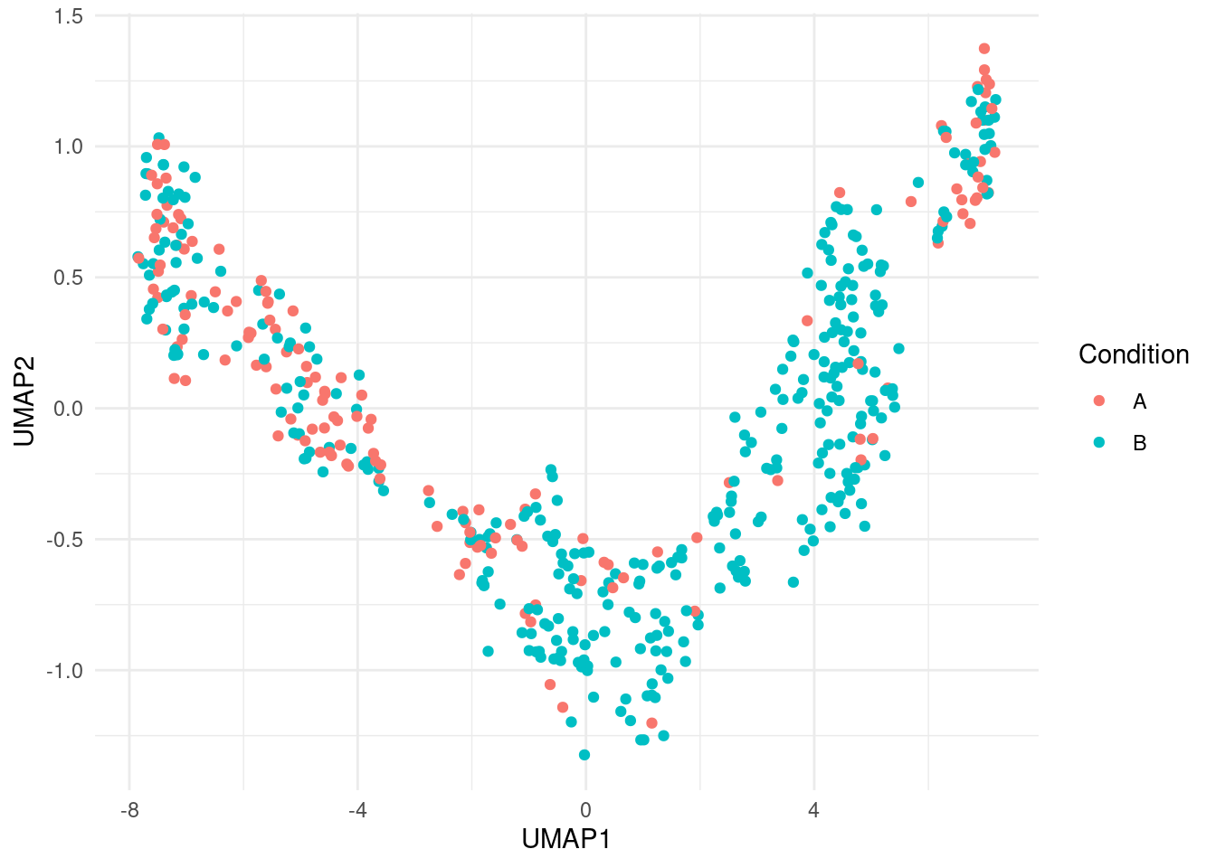
Milo object
traj_milo <- Milo(traj_sce)
reducedDim(traj_milo, "UMAP") <- reducedDim(traj_sce, "UMAP")

traj_milo
class: Milo
dim: 500 500
metadata(0):
assays(2): counts logcounts
rownames(500): G1 G2 ... G499 G500
rowData names(0):
colnames(500): C1 C2 ... C499 C500
colData names(5): cell_id group_id Condition Replicate Sample
reducedDimNames(2): PCA UMAP
mainExpName: NULL
altExpNames(0):
nhoods dimensions(2): 1 1
nhoodCounts dimensions(2): 1 1
nhoodDistances dimension(1): 0
graph names(0):
nhoodIndex names(1): 0
nhoodExpression dimension(2): 1 1
nhoodReducedDim names(0):
nhoodGraph names(0):
nhoodAdjacency dimension(2): 1 1Construct KNN graph
traj_milo <- buildGraph(traj_milo, k = 10, d = 30)Constructing kNN graph with k:10Defining representative neighbourhoods
traj_milo <- makeNhoods(traj_milo, prop = 0.1, k = 10, d=30, refined = TRUE)Checking valid objectRunning refined sampling with reduced_dimplotNhoodSizeHist(traj_milo)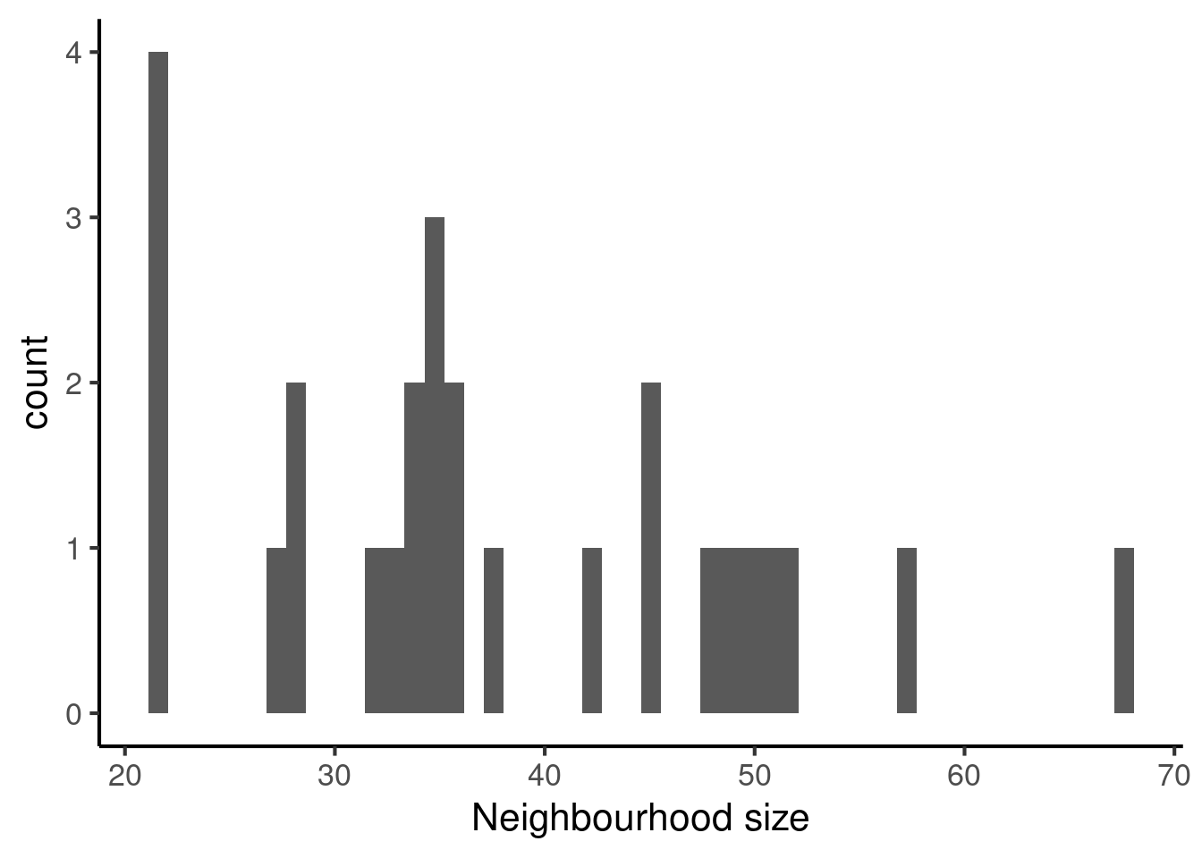
Counting cells in neighbourhoods
traj_milo <- countCells(traj_milo, meta.data = data.frame(colData(traj_milo)), samples="Sample")Checking meta.data validityCounting cells in neighbourhoodshead(nhoodCounts(traj_milo))6 x 6 sparse Matrix of class "dgCMatrix"
B_R1 A_R1 A_R2 B_R2 B_R3 A_R3
1 15 . 1 22 29 1
2 8 . . 14 28 1
3 9 6 7 7 6 10
4 13 2 1 19 21 1
5 5 6 4 8 6 7
6 6 7 5 12 8 11Differential abundance testing
traj_design <- data.frame(colData(traj_milo))[,c("Sample", "Condition")]
traj_design <- distinct(traj_design)
rownames(traj_design) <- traj_design$Sample
## Reorder rownames to match columns of nhoodCounts(milo)
traj_design <- traj_design[colnames(nhoodCounts(traj_milo)), , drop=FALSE]

traj_design
Sample Condition
B_R1 B_R1 B
A_R1 A_R1 A
A_R2 A_R2 A
B_R2 B_R2 B
B_R3 B_R3 B
A_R3 A_R3 Atraj_milo <- calcNhoodDistance(traj_milo, d=30)'as(<dgTMatrix>, "dgCMatrix")' is deprecated.
Use 'as(., "CsparseMatrix")' instead.
See help("Deprecated") and help("Matrix-deprecated").da_results <- testNhoods(traj_milo, design = ~ Condition, design.df = traj_design)Using TMM normalisationRunning with model contrastsPerforming spatial FDR correction with k-distance weightingda_results %>%
dplyr::arrange(SpatialFDR) %>%
head() logFC logCPM F PValue FDR Nhood SpatialFDR
1 3.886596 16.30369 33.87551 6.099827e-08 1.646953e-06 1 1.611592e-06
2 4.337415 15.95908 29.07187 4.140178e-07 5.589241e-06 2 5.504741e-06
4 2.655301 16.09039 19.26657 2.658333e-05 2.392499e-04 4 2.371232e-04
8 2.897422 15.53655 20.75784 6.887852e-05 4.649300e-04 8 4.627806e-04
24 -1.527532 15.73713 29.71687 5.308236e-04 2.866447e-03 24 2.872952e-03
23 2.278126 15.50551 10.21171 1.830055e-03 8.235247e-03 23 8.283248e-03Visualise neighbourhoods displaying DA
traj_milo <- buildNhoodGraph(traj_milo)

my_umap + plotNhoodGraphDA(traj_milo, da_results, alpha=0.05) +
  plot_layout(guides="collect")
Adding nhood effect sizes to neighbourhood graph attributes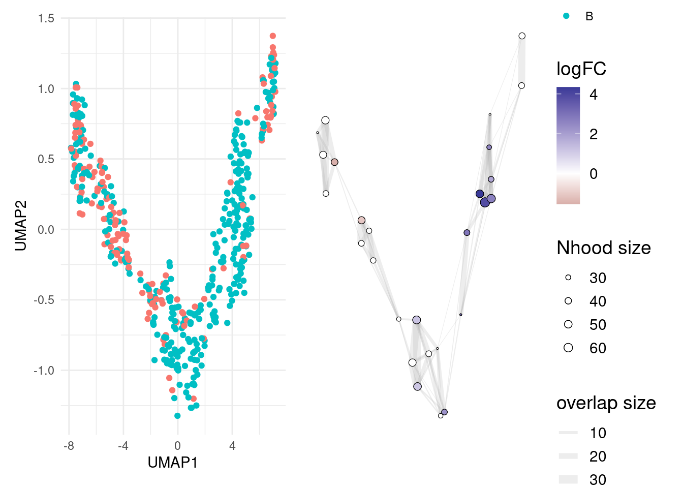
Mouse gastrulation example
Data
4 samples at stage E7 and 4 samples at stage E7.5.
select_samples <- c(2,  3,  6, 4, #15,
                    # 19,
                    10, 14#, 20 #30
                    #31, 32
                    )
EmbryoAtlasData(samples = select_samples) |>
  suppressMessages() |>
  suppressWarnings() -> embryo_data

embryo_data
class: SingleCellExperiment
dim: 29452 7558
metadata(0):
assays(1): counts
rownames(29452): ENSMUSG00000051951 ENSMUSG00000089699 ...
ENSMUSG00000096730 ENSMUSG00000095742
rowData names(2): ENSEMBL SYMBOL
colnames(7558): cell_361 cell_362 ... cell_29013 cell_29014
colData names(17): cell barcode ... colour sizeFactor
reducedDimNames(2): pca.corrected umap
mainExpName: NULL
altExpNames(0):Visualise the data
We will test for significant differences in abundance of cells between two stages of development.
embryo_data <- embryo_data[,apply(reducedDim(embryo_data, "pca.corrected"), 1, function(x) !all(is.na(x)))]
embryo_data <- runUMAP(embryo_data, dimred = "pca.corrected", name = 'umap')

plotReducedDim(embryo_data, colour_by="stage", dimred = "umap") 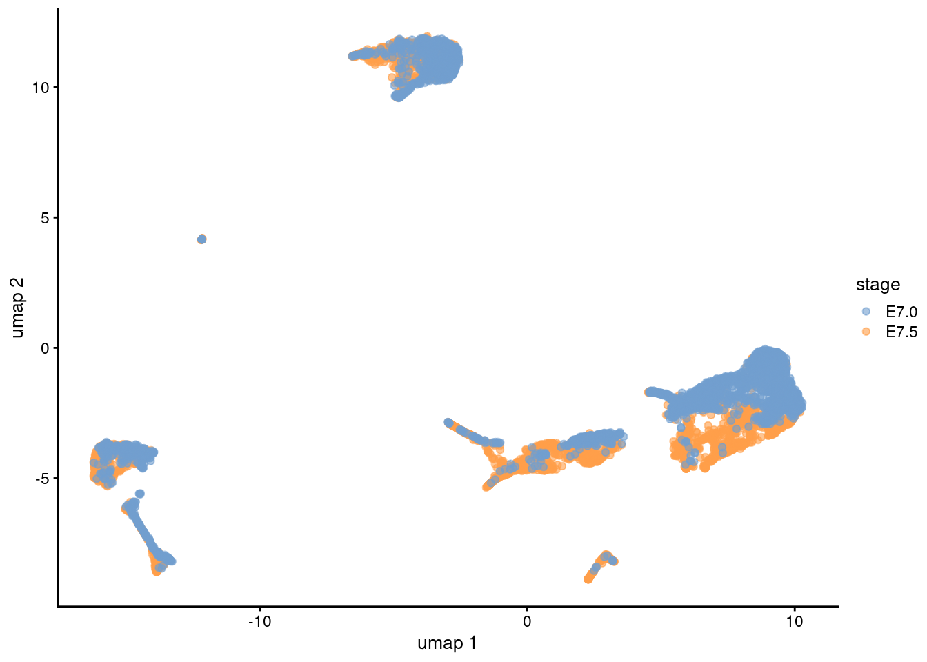
| Version | Author | Date |
|---|---|---|
| bb9a8b6 | Dave Tang | 2025-01-11 |
Create a Milo object
For differential abundance analysis on graph neighbourhoods we first
construct a Milo object. This extends the
SingleCellExperiment class to store information about
neighbourhoods on the KNN graph.
embryo_milo <- Milo(embryo_data)
embryo_milo
class: Milo
dim: 29452 6875
metadata(0):
assays(1): counts
rownames(29452): ENSMUSG00000051951 ENSMUSG00000089699 ...
ENSMUSG00000096730 ENSMUSG00000095742
rowData names(2): ENSEMBL SYMBOL
colnames(6875): cell_361 cell_362 ... cell_29013 cell_29014
colData names(17): cell barcode ... colour sizeFactor
reducedDimNames(2): pca.corrected umap
mainExpName: NULL
altExpNames(0):
nhoods dimensions(2): 1 1
nhoodCounts dimensions(2): 1 1
nhoodDistances dimension(1): 0
graph names(0):
nhoodIndex names(1): 0
nhoodExpression dimension(2): 1 1
nhoodReducedDim names(0):
nhoodGraph names(0):
nhoodAdjacency dimension(2): 1 1Construct KNN graph
The {miloR} package includes functionality to build and store the
graph from the PCA dimensions stored in the reducedDim
slot. For graph building you need to define a few parameters:
d: the number of reduced dimensions to use for KNN refinement. We recommend using the same d used for KNN graph building, or to select PCs by inspecting the scree plot.k: this affects the power of DA testing, since we need to have enough cells from each sample represented in a neighbourhood to estimate the variance between replicates. On the other side, increasingktoo much might lead to over-smoothing. We suggest to start by using the same value forkused for KNN graph building for clustering and UMAP visualization. We will later use some heuristics to evaluate whether the value ofkshould be increased.
embryo_milo <- buildGraph(embryo_milo, k = 30, d = 30, reduced.dim = "pca.corrected")Constructing kNN graph with k:30Defining representative neighbourhoods on the KNN graph
We define the neighbourhood of a cell, the index, as the group of cells connected by an edge in the KNN graph to the index cell. For efficiency, DA testing is performed on a sample of indices containing a subset of representative cells, using a KNN sampling algorithm used by Gut et al. 2015.
As well as d and k, for sampling we need to
define a few additional parameters:
prop: the proportion of cells to randomly sample to start with. We suggest usingprop=0.1for datasets of less than 30k cells. For bigger datasets usingprop=0.05should be sufficient (and makes computation faster).refined: indicates whether you want to use the sampling refinement algorithm, or just pick cells at random. The default and recommended way to go is to use refinement. The only situation in which you might consider using random instead, is if you have batch corrected your data with a graph based correction algorithm, such as BBKNN, but the results of DA testing will be suboptimal.
Once we have defined neighbourhoods, we plot the distribution of
neighbourhood sizes (i.e. how many cells form each neighbourhood) to
evaluate whether the value of k used for graph building was
appropriate. We can check this out using the
plotNhoodSizeHist() function.
As a rule of thumb we want to have an average neighbourhood size over 5 x N_samples.
embryo_milo <- makeNhoods(embryo_milo, prop = 0.1, k = 30, d=30, refined = TRUE, reduced_dims = "pca.corrected")Checking valid objectRunning refined sampling with reduced_dimplotNhoodSizeHist(embryo_milo)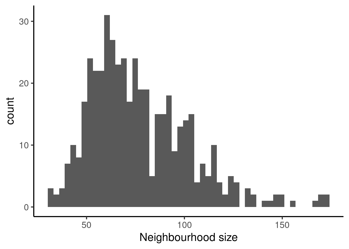
| Version | Author | Date |
|---|---|---|
| bb9a8b6 | Dave Tang | 2025-01-11 |
Counting cells in neighbourhoods
Milo leverages the variation in cell numbers between replicates for the same experimental condition to test for differential abundance. Therefore we have to count how many cells from each sample are in each neighbourhood. We need to use the cell metadata and specify which column contains the sample information.
This adds to the Milo object a \(n \times m\) matrix, where \(n\) is the number of neighbourhoods and \(m\) is the number of experimental samples. Values indicate the number of cells from each sample counted in a neighbourhood. This count matrix will be used for DA testing.
embryo_milo <- countCells(embryo_milo, meta.data = as.data.frame(colData(embryo_milo)), sample="sample")Checking meta.data validityCounting cells in neighbourhoodshead(nhoodCounts(embryo_milo))6 x 6 sparse Matrix of class "dgCMatrix"
2 3 6 4 10 14
1 . 2 24 2 11 .
2 1 4 48 7 25 6
3 3 4 87 5 15 11
4 . . 5 . 90 19
5 . . 27 . 47 7
6 11 5 26 2 . .Defining experimental design
Now we are all set to test for differential abundance in neighbourhoods. We implement this hypothesis testing in a generalized linear model (GLM) framework, specifically using the Negative Binomial GLM implementation in {edgeR}.
embryo_design <- data.frame(colData(embryo_milo))[,c("sample", "stage", "sequencing.batch")]

## Convert batch info from integer to factor
embryo_design$sequencing.batch <- as.factor(embryo_design$sequencing.batch)
embryo_design <- distinct(embryo_design)
rownames(embryo_design) <- embryo_design$sample

embryo_design
sample stage sequencing.batch
2 2 E7.5 1
3 3 E7.5 1
6 6 E7.5 1
4 4 E7.5 1
10 10 E7.0 1
14 14 E7.0 2Computing neighbourhood connectivity
Milo uses an adaptation of the Spatial FDR correction introduced by
cydar, where we correct p-values accounting for the amount of overlap
between neighbourhoods. Specifically, each hypothesis test P-value is
weighted by the reciprocal of the \(k\)th nearest neighbour distance. To use
this statistic we first need to store the distances between nearest
neighbors in the Milo object. This is done by the
calcNhoodDistance() function (N.B. this step is the most
time consuming of the analysis workflow and might take a couple of
minutes for large datasets).
embryo_milo <- calcNhoodDistance(embryo_milo, d=30, reduced.dim = "pca.corrected")Testing
Now we can do the DA test, explicitly defining our experimental design. In this case, we want to test for differences between experimental stages, while accounting for the variability between technical batches.
This calculates a Fold-change and corrected P-value for each neighbourhood, which indicates whether there is significant differential abundance between developmental stages. The main statistics we consider here are:
logFC: indicates the log-Fold change in cell numbers between samples from E7.5 and samples from E7.0.PValue: reports P-values before FDR correction.SpatialFDR: reports P-values corrected for multiple testing accounting for overlap between neighbourhoods.
da_results <- testNhoods(embryo_milo, design = ~ sequencing.batch + stage, design.df = embryo_design, reduced.dim="pca.corrected")Using TMM normalisationRunning with model contrastsPerforming spatial FDR correction with k-distance weightingda_results |>
arrange(SpatialFDR) |>
head() logFC logCPM F PValue FDR Nhood SpatialFDR
36 -8.702572 11.38854 51.62516 1.091251e-12 5.063407e-10 36 3.911834e-10
377 -8.791174 11.72929 47.66587 7.658840e-12 1.776851e-09 377 1.394183e-09
314 -7.170721 11.85656 45.98225 1.758371e-11 2.039710e-09 314 1.593529e-09
347 -8.426464 11.27041 46.53411 1.338823e-11 2.039710e-09 347 1.593529e-09
52 -7.838842 12.18774 44.65865 3.383398e-11 3.139793e-09 52 2.453204e-09
223 -6.168287 11.96552 42.75561 8.685459e-11 6.566003e-09 223 5.087165e-09Confirming that each test was on the number of neighbourhoods.
nrow(nhoodCounts(embryo_milo)) == nrow(da_results)[1] TRUEReturns a list of the single-cells that are the neighbourhood indices.
unlist(nhoodIndex(embryo_milo)) [1] 3265 2172 3219 4391 5208 521 4942 3360 3894 1683 4574 2019 5549 982 2111
[16] 2065 2681 2179 2117 1970 4874 2309 4114 1188 3739 1819 4837 3163 3907 5444
[31] 1607 1267 4276 2326 5312 4476 6373 5039 1686 4509 5077 1066 1849 4839 1155
[46] 5200 3135 2746 730 3770 4842 3930 4285 906 4836 1357 5591 6500 1573 5650
[61] 2619 3231 2080 2331 4587 2090 4763 3050 1374 1324 5093 1919 4599 3685 2716
[76] 1195 1141 2741 2616 958 4795 3655 6674 3115 1742 813 1017 2505 774 1510
[91] 5670 2296 5613 1100 2958 4500 6524 5104 5354 3849 5375 5004 2464 3926 4010
[106] 2051 3382 5930 2661 893 2106 778 1151 4749 2974 782 1039 4829 2906 2412
[121] 5331 4548 2710 2456 4339 4414 4497 1168 1217 1072 3565 2664 2034 1286 1373
[136] 995 1793 2835 1675 1450 4472 4547 915 2745 3670 2248 2268 874 4866 5495
[151] 1606 4596 3949 3139 1649 2815 1091 2795 3782 42 2005 1545 2970 2588 5172
[166] 6823 3348 4229 3527 2501 5413 907 4439 2999 1043 2586 6000 343 3563 4954
[181] 751 875 4800 3395 3626 1462 4542 3241 1984 4460 2804 2581 2561 547 3595
[196] 2148 2901 1477 3844 321 4728 3013 3221 3694 2275 6699 1626 4332 4171 4182
[211] 1795 3836 2787 3067 5344 1778 1494 5566 4333 849 3568 4796 4446 1472 5147
[226] 2744 2471 4457 4868 1144 2673 3814 3202 1671 2378 2176 4824 2398 2556 500
[241] 6425 5357 2547 2803 2987 1897 1947 1651 832 2578 2192 6751 1124 3267 2675
[256] 4308 5573 1005 4775 5292 1210 4445 3085 1161 4173 6399 2698 3577 1130 4903
[271] 1811 5515 2610 2980 2539 2383 5286 2062 6183 5873 5291 1122 831 4880 4622
[286] 2194 747 4106 1074 1816 4679 4338 1175 5035 2925 4929 1299 2018 113 1818
[301] 5758 2482 5139 4527 3740 2325 4610 2351 6155 4946 860 1871 2411 4083 5995
[316] 5213 965 1951 5405 4822 6565 1215 3924 2393 4511 4012 5400 1636 2349 1505
[331] 2196 889 2690 2141 4882 3093 4634 5516 1998 4084 2110 825 1765 3725 2212
[346] 3596 4873 6273 2435 3776 1764 4427 4759 1752 2274 4362 3072 4317 5525 1306
[361] 4245 1111 1530 3779 1086 3681 3164 2749 4856 2968 4751 2445 3098 5290 1046
[376] 2321 3554 4456 5135 3051 2036 5266 329 4040 4926 4350 4780 4740 5677 4920
[391] 2253 3815 2490 5128 5578 3792 2866 4898 5027 2487 2643 841 2990 5338 311
[406] 3154 5311 3569 2373 5011 604 1076 5548 5029 3911 1090 2208 5236 128 4919
[421] 1136 2606 1127 2772 6532 2343 1729 2808 5730 4167 3349 5179 2984 490 2064
[436] 2059 894 3047 1238 5610 1469 1218 2986 495 2971 5611 1169 2218 5096 703
[451] 2388 2128 2627 2771 892 2967 2878 4879 4148 923 1196 4708 4313 2104Returns a sparse matrix of \(C \times N\) mapping of \(C\) single-cells to \(N\) neighbourhoods.
dim(nhoods(embryo_milo))[1] 6875 464Returns a list of sparse matrix of cell-to-cell distances between nearest neighbours, one list entry per neighbourhood. Largely used internally for computing the k-distance weighting in graphSpatialFDR.
Can be used to get the cells that belong to a neighbourhood.
n_dists <- nhoodDistances(embryo_milo)
rownames(n_dists[[1]])
[1] "cell_963" "cell_1044" "cell_2734" "cell_2804" "cell_3119"
[6] "cell_3294" "cell_3491" "cell_3519" "cell_3594" "cell_3900"
[11] "cell_3944" "cell_4061" "cell_4184" "cell_4229" "cell_4248"
[16] "cell_4479" "cell_4482" "cell_4543" "cell_4624" "cell_4940"
[21] "cell_5223" "cell_5246" "cell_5260" "cell_5273" "cell_5414"
[26] "cell_5452" "cell_1290" "cell_1394" "cell_13973" "cell_14359"
[31] "cell_14842" "cell_14862" "cell_14909" "cell_15069" "cell_15250"
[36] "cell_15461" "cell_15674" "cell_15990" "cell_16313"Check.
nhoodCounts(embryo_milo) |> Matrix::rowSums() -> a
purrr::map_int(n_dists, nrow) -> b

all(a == b)
[1] TRUEMost significant neighbourhood is that is composed of cells entirely in one stage.
da_results |>
  dplyr::slice_min(order_by = SpatialFDR, n = 1) |>
  rownames() |>
  as.numeric() -> most_signif_nhood

n_dists[[most_signif_nhood]] |>
  rownames() -> most_signif_nhood_cells

my_subset <- embryo_data[, most_signif_nhood_cells]

aggregateAcrossCells(my_subset, ids = colData(my_subset)$stage)
class: SingleCellExperiment
dim: 29452 1
metadata(0):
assays(1): counts
rownames(29452): ENSMUSG00000051951 ENSMUSG00000089699 ...
ENSMUSG00000096730 ENSMUSG00000095742
rowData names(2): ENSEMBL SYMBOL
colnames(1): E7.0
colData names(19): cell barcode ... ids ncells
reducedDimNames(2): pca.corrected umap
mainExpName: NULL
altExpNames(0):table(colData(my_subset)$stage)
E7.0
  70
Plot most significant.
reducedDim(embryo_data, "umap") |>
  as.data.frame() -> umap_coords

umap_coords$most_signif <- rownames(umap_coords) %in% most_signif_nhood_cells

ggplot(umap_coords, aes(UMAP1, UMAP2)) +
  geom_point() +
  theme_minimal() +
  facet_grid(~most_signif)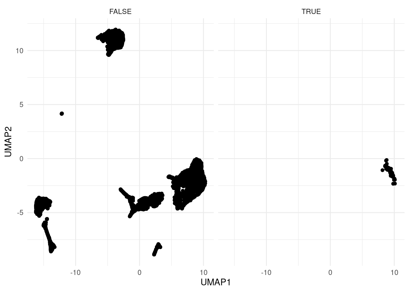
Inspecting DA testing results
We can start inspecting the results of our DA analysis from a couple of standard diagnostic plots. We first inspect the distribution of uncorrected P values, to verify that the test was balanced.
ggplot(da_results, aes(PValue)) + geom_histogram(bins=50)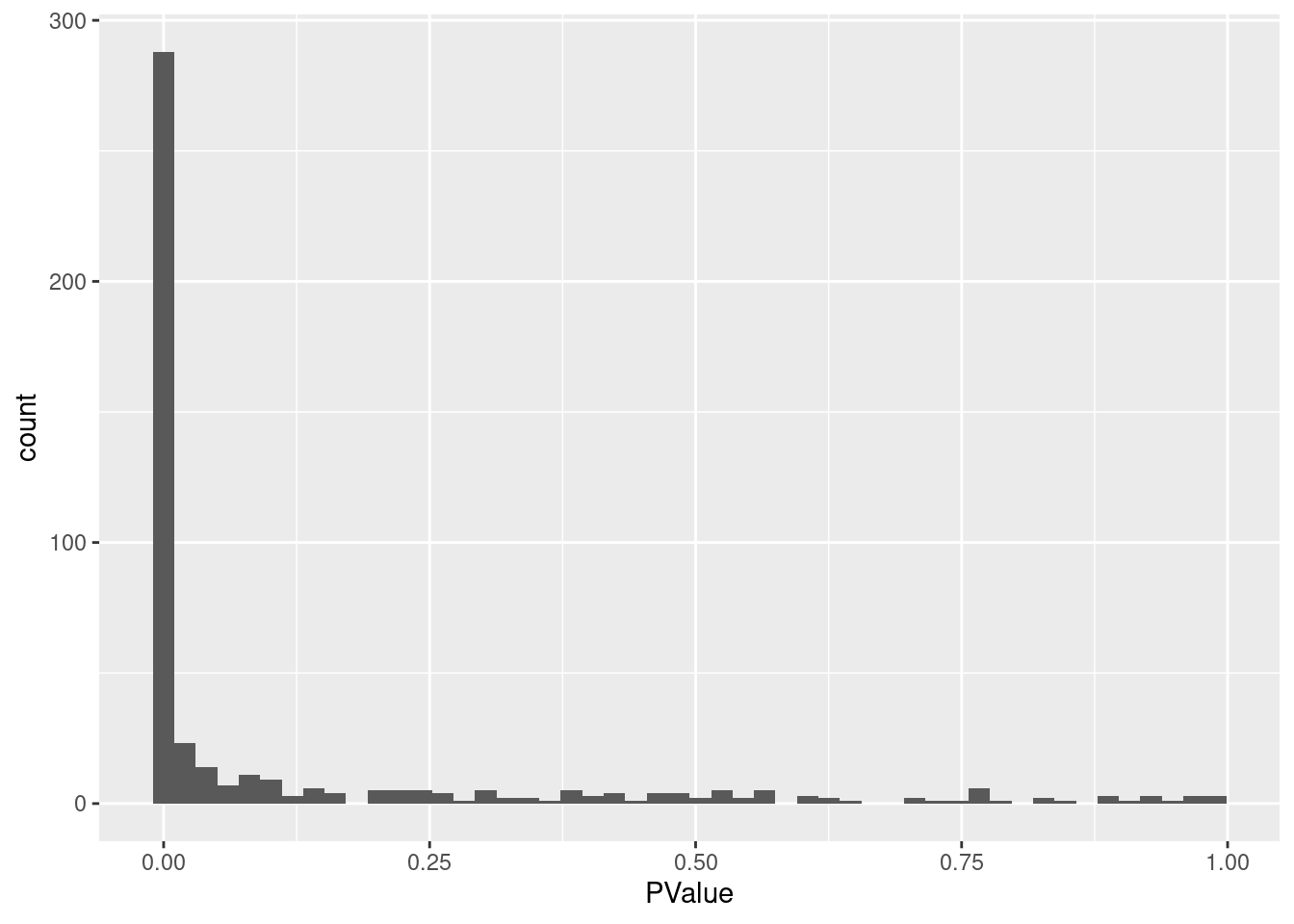
| Version | Author | Date |
|---|---|---|
| bb9a8b6 | Dave Tang | 2025-01-11 |
Then we visualize the test results with a volcano plot (remember that each point here represents a neighbourhood, not a cell).
ggplot(da_results, aes(logFC, -log10(SpatialFDR))) +
  geom_point() +
  geom_hline(yintercept = 1) ## Mark significance threshold (10% FDR)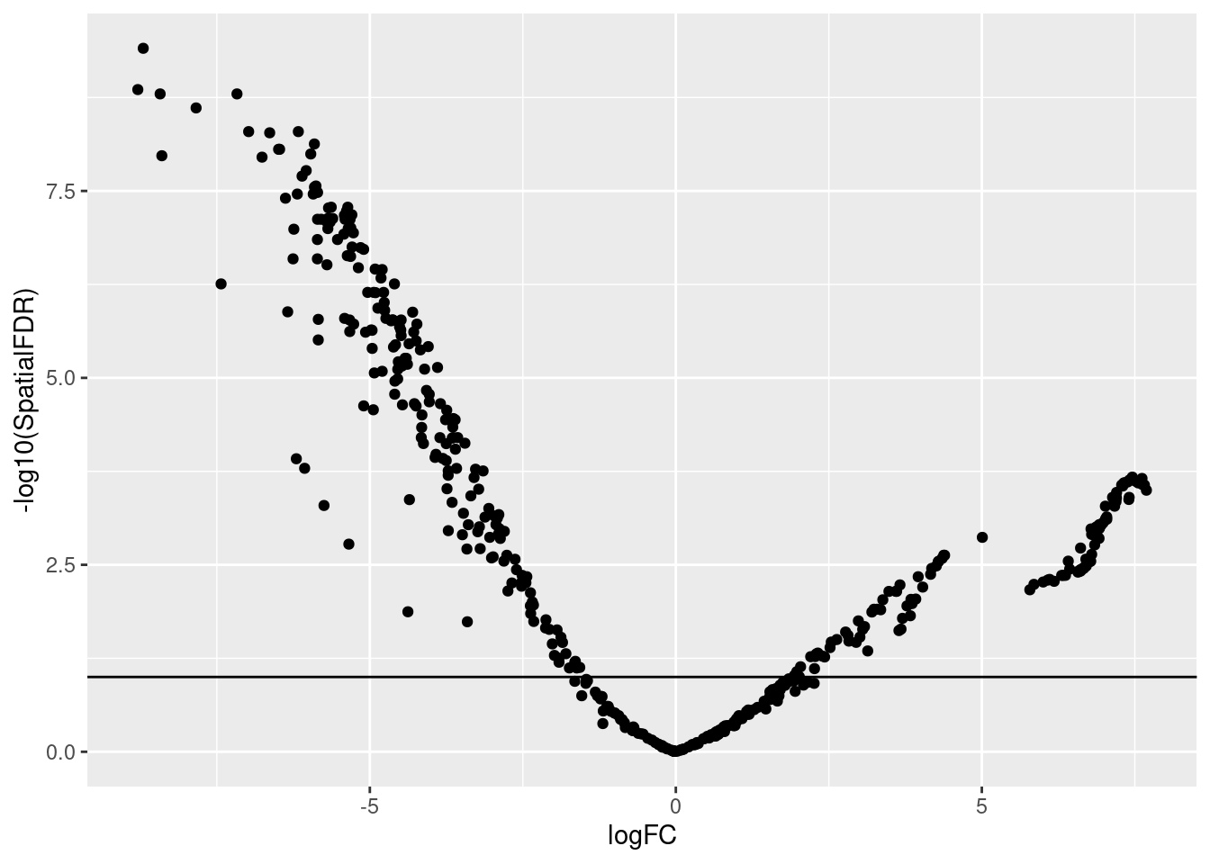
| Version | Author | Date |
|---|---|---|
| bb9a8b6 | Dave Tang | 2025-01-11 |
To visualise DA results relating them to the embedding of single cells, we can build an abstracted graph of neighbourhoods that we can superimpose on the single-cell embedding. Here each node represents a neighbourhood, while edges indicate how many cells two neighbourhoods have in common. Here the layout of nodes is determined by the position of the index cell in the UMAP embedding of all single-cells. The neighbourhoods displaying significant DA are colored by their log-Fold Change.
embryo_milo <- buildNhoodGraph(embryo_milo)

## Plot single-cell UMAP
umap_pl <- plotReducedDim(embryo_milo, dimred = "umap", colour_by="stage", text_by = "celltype",
                          text_size = 3, point_size=0.5) +
  guides(fill="none")

## Plot neighbourhood graph
nh_graph_pl <- plotNhoodGraphDA(embryo_milo, da_results, layout="umap",alpha=0.1)
Adding nhood effect sizes to neighbourhood graph attributesumap_pl + nh_graph_pl +
plot_layout(guides="collect")Warning: ggrepel: 19 unlabeled data points (too many overlaps). Consider
increasing max.overlaps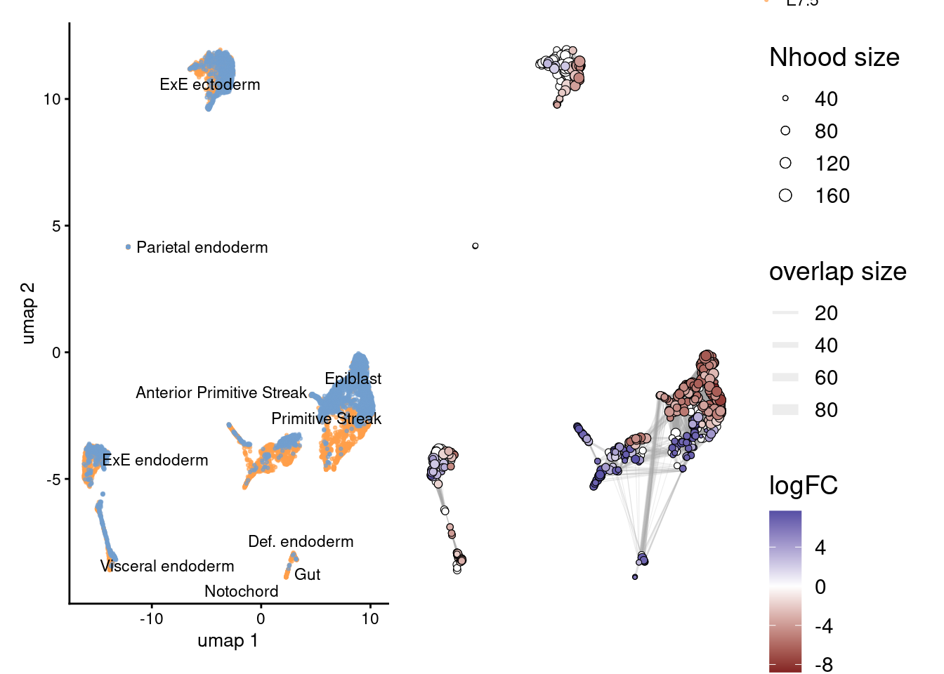
| Version | Author | Date |
|---|---|---|
| bb9a8b6 | Dave Tang | 2025-01-11 |
We might also be interested in visualising whether DA is particularly
evident in certain cell types. To do this, we assign a cell type label
to each neighbourhood by finding the most abundant cell type within
cells in each neighbourhood. We can label neighbourhoods in the results
data.frame using the function annotateNhoods.
This also saves the fraction of cells harbouring the label.
da_results <- annotateNhoods(embryo_milo, da_results, coldata_col = "celltype")Converting celltype to factor...head(da_results) logFC logCPM F PValue FDR Nhood SpatialFDR
1 -0.7073196 10.38623 0.5596000 4.545478e-01 5.131635e-01 1 5.170902e-01
2 -0.6852005 11.51879 0.6659869 4.145939e-01 4.749915e-01 2 4.773720e-01
3 0.4505361 11.73195 0.2354735 6.275710e-01 6.694091e-01 3 6.705023e-01
4 -6.0397103 12.02021 38.5362677 7.078557e-10 2.189634e-08 4 1.690890e-08
5 -3.1492070 11.32228 16.2297553 5.913724e-05 1.932372e-04 5 1.756735e-04
6 6.7795549 10.89194 10.2510770 1.396926e-03 2.842866e-03 6 2.831445e-03
celltype celltype_fraction
1 Parietal endoderm 1.000000
2 Primitive Streak 0.956044
3 ExE ectoderm 1.000000
4 Epiblast 0.754386
5 ExE ectoderm 1.000000
6 Caudal epiblast 0.750000While neighbourhoods tend to be homogeneous, we can define a threshold for celltype_fraction to exclude neighbourhoods that are a mix of cell types.
ggplot(da_results, aes(celltype_fraction)) + geom_histogram(bins=50)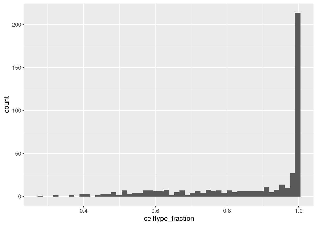
| Version | Author | Date |
|---|---|---|
| bb9a8b6 | Dave Tang | 2025-01-11 |
Now we can visualise the distribution of DA Fold Changes in different cell types.
da_results$celltype <- ifelse(da_results$celltype_fraction < 0.7, "Mixed", da_results$celltype)

plotDAbeeswarm(da_results, group.by = "celltype")
Converting group_by to factor...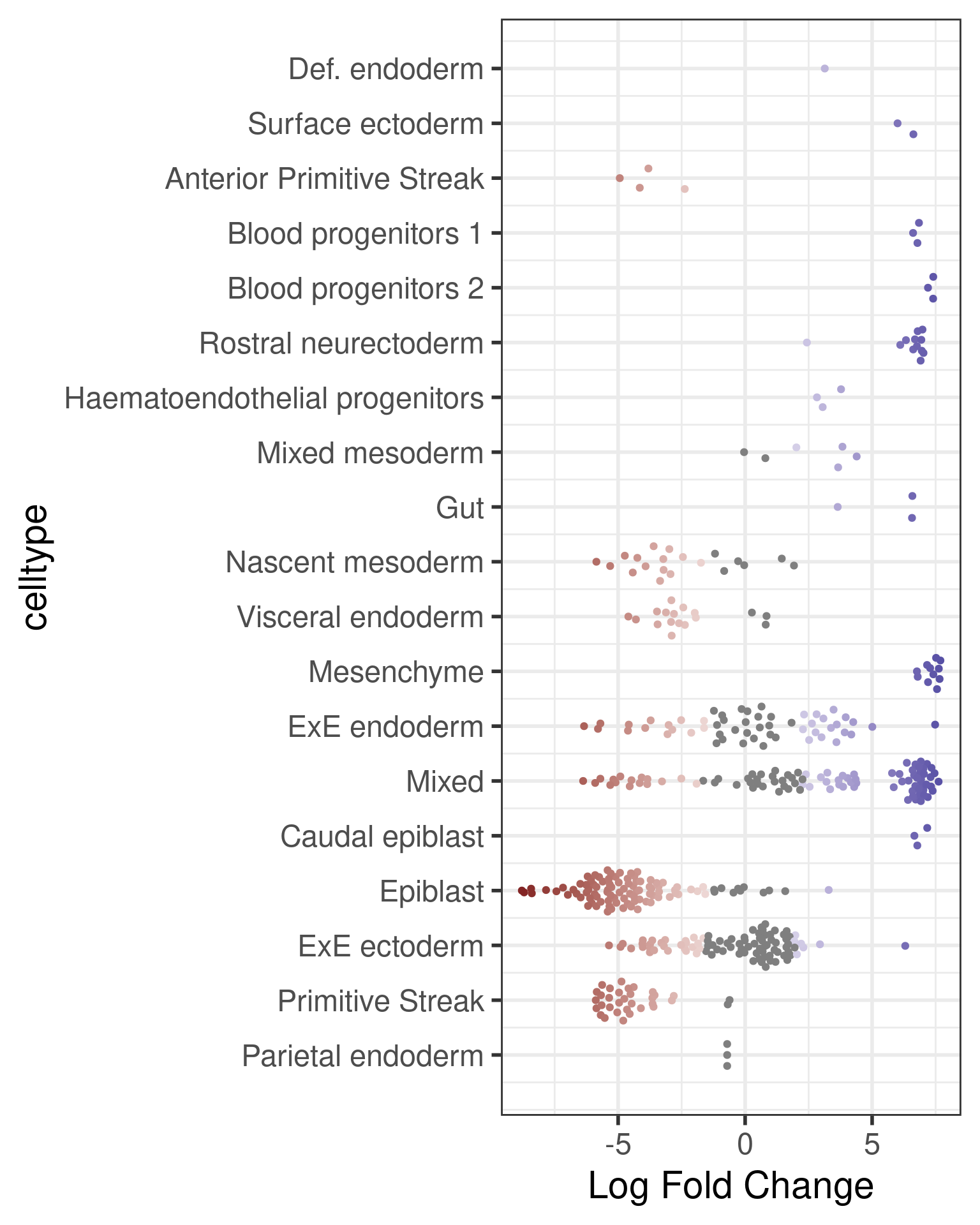
| Version | Author | Date |
|---|---|---|
| bb9a8b6 | Dave Tang | 2025-01-11 |
This is already quite informative: we can see that certain early development cell types, such as epiblast and primitive streak, are enriched in the earliest time stage, while others are enriched later in development, such as ectoderm cells. Interestingly, we also see plenty of DA neighbourhood with a mixed label. This could indicate that transitional states show changes in abundance in time.
Finding markers of DA populations
Once you have found your neighbourhoods showing significant DA
between conditions, you might want to find gene signatures specific to
the cells in those neighbourhoods. The function
findNhoodGroupMarkers() runs a one-VS-all differential gene
expression test to identify marker genes for a group of neighbourhoods
of interest. Before running this function you will need to define your
neighbourhood groups depending on your biological question, that need to
be stored as a NhoodGroup column in the
da_results data.frame.
## Add log normalized count to Milo object
embryo_milo <- logNormCounts(embryo_milo)

da_results$NhoodGroup <- as.numeric(da_results$SpatialFDR < 0.1 & da_results$logFC < 0)
da_nhood_markers <- findNhoodGroupMarkers(embryo_milo, da_results, subset.row = rownames(embryo_milo)[1:10])
Warning: Zero sample variances detected, have been offset away from zero
Warning: Zero sample variances detected, have been offset away from zerohead(da_nhood_markers) GeneID logFC_0 adj.P.Val_0 logFC_1 adj.P.Val_1
1 ENSMUSG00000025900 9.299023e-05 1.000000e+00 -9.299023e-05 1.000000e+00
2 ENSMUSG00000025902 1.130534e-01 9.610514e-06 -1.130534e-01 9.610514e-06
3 ENSMUSG00000025903 -6.605353e-02 4.487599e-03 6.605353e-02 4.487599e-03
4 ENSMUSG00000033813 -6.175050e-02 8.928182e-03 6.175050e-02 8.928182e-03
5 ENSMUSG00000033845 -6.025957e-02 1.563741e-02 6.025957e-02 1.563741e-02
6 ENSMUSG00000051951 0.000000e+00 1.000000e+00 0.000000e+00 1.000000e+00da_nhood_markers <- findNhoodGroupMarkers(embryo_milo, da_results, subset.row = rownames(embryo_milo)[1:10],
aggregate.samples = TRUE, sample_col = "sample")Warning: Zero sample variances detected, have been offset away from zero
Warning: Zero sample variances detected, have been offset away from zerohead(da_nhood_markers) GeneID logFC_0 adj.P.Val_0 logFC_1 adj.P.Val_1
1 ENSMUSG00000025900 0.001765224 1 -0.001765224 1
2 ENSMUSG00000025902 -0.205886718 1 0.205886718 1
3 ENSMUSG00000025903 -0.010020237 1 0.010020237 1
4 ENSMUSG00000033813 -0.050052716 1 0.050052716 1
5 ENSMUSG00000033845 -0.168226202 1 0.168226202 1
6 ENSMUSG00000051951 0.000000000 1 0.000000000 1Automatic grouping of neighbourhoods
## Run buildNhoodGraph to store nhood adjacency matrix
embryo_milo <- buildNhoodGraph(embryo_milo)

## Find groups
da_results <- groupNhoods(embryo_milo, da_results, max.lfc.delta = 10)
Found 332 DA neighbourhoods at FDR 10%nhoodAdjacency found - using for nhood groupinghead(da_results) logFC logCPM F PValue FDR Nhood SpatialFDR
1 -0.7073196 10.38623 0.5596000 4.545478e-01 5.131635e-01 1 5.170902e-01
2 -0.6852005 11.51879 0.6659869 4.145939e-01 4.749915e-01 2 4.773720e-01
3 0.4505361 11.73195 0.2354735 6.275710e-01 6.694091e-01 3 6.705023e-01
4 -6.0397103 12.02021 38.5362677 7.078557e-10 2.189634e-08 4 1.690890e-08
5 -3.1492070 11.32228 16.2297553 5.913724e-05 1.932372e-04 5 1.756735e-04
6 6.7795549 10.89194 10.2510770 1.396926e-03 2.842866e-03 6 2.831445e-03
celltype celltype_fraction NhoodGroup
1 Parietal endoderm 1.000000 1
2 Primitive Streak 0.956044 2
3 ExE ectoderm 1.000000 3
4 Epiblast 0.754386 4
5 ExE ectoderm 1.000000 3
6 Caudal epiblast 0.750000 5plotNhoodGroups(embryo_milo, da_results, layout="umap") 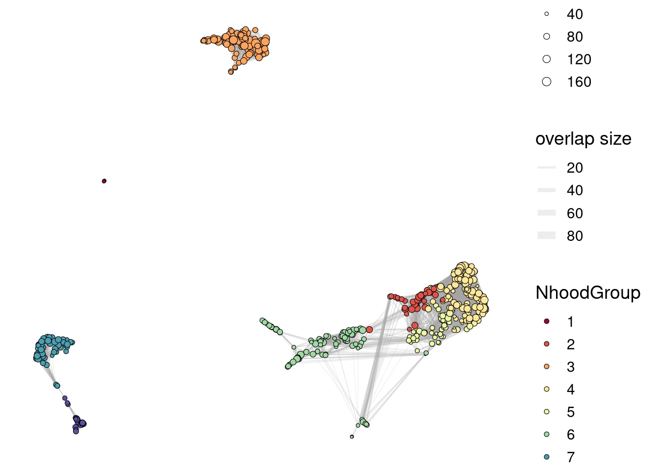
| Version | Author | Date |
|---|---|---|
| bb9a8b6 | Dave Tang | 2025-01-11 |
plotDAbeeswarm(da_results, "NhoodGroup")Converting group_by to factor...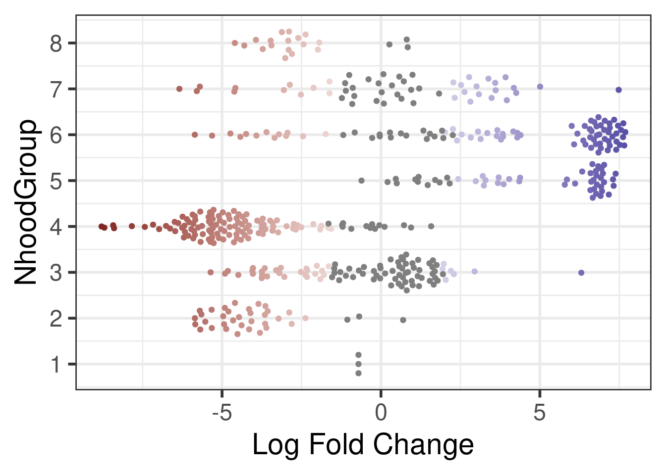
| Version | Author | Date |
|---|---|---|
| bb9a8b6 | Dave Tang | 2025-01-11 |
set.seed(42)
da_results <- groupNhoods(embryo_milo, da_results, max.lfc.delta = 10, overlap=1)
Found 332 DA neighbourhoods at FDR 10%nhoodAdjacency found - using for nhood groupingplotNhoodGroups(embryo_milo, da_results, layout="umap")
| Version | Author | Date |
|---|---|---|
| bb9a8b6 | Dave Tang | 2025-01-11 |
Finding gene signatures for neighbourhoods
## Exclude zero counts genes
keep.rows <- rowSums(logcounts(embryo_milo)) != 0
embryo_milo <- embryo_milo[keep.rows, ]

## Find HVGs
set.seed(101)
dec <- modelGeneVar(embryo_milo)
hvgs <- getTopHVGs(dec, n=2000)

# this vignette randomly fails to identify HVGs for some reason
if(!length(hvgs)){
    set.seed(42)
    dec <- modelGeneVar(embryo_milo)
    hvgs <- getTopHVGs(dec, n=2000)
}

head(hvgs)
[1] "ENSMUSG00000032083" "ENSMUSG00000095180" "ENSMUSG00000061808"
[4] "ENSMUSG00000002985" "ENSMUSG00000024990" "ENSMUSG00000024391"set.seed(42)
nhood_markers <- findNhoodGroupMarkers(embryo_milo, da_results, subset.row = hvgs,
aggregate.samples = TRUE, sample_col = "sample")
head(nhood_markers) GeneID logFC_1 adj.P.Val_1 logFC_2 adj.P.Val_2 logFC_3
1 ENSMUSG00000000031 -0.1957851 9.023691e-01 -1.6227811 0.131661210 1.0818991
2 ENSMUSG00000000078 1.3761092 4.763130e-07 -0.7577163 0.027746376 -0.1254065
3 ENSMUSG00000000088 0.8440478 1.708425e-02 -0.2230027 0.542175995 -0.2398095
4 ENSMUSG00000000125 -0.3215022 1.333035e-01 0.4961217 0.006035858 -0.1759920
5 ENSMUSG00000000149 0.1267912 5.214792e-01 -0.0666690 0.674509763 -0.1369532
6 ENSMUSG00000000184 -0.9431346 1.760344e-01 0.6236021 0.330231952 -0.9388169
adj.P.Val_3 logFC_4 adj.P.Val_4 logFC_5 adj.P.Val_5 logFC_6
1 0.23946003 -1.6554796 0.1458825 -1.80398024 0.1388493 -0.89469039
2 0.67224856 -0.1319154 0.6784129 -0.15102950 0.6054605 0.02395376
3 0.41954806 -0.3931160 0.3057337 -0.32144387 0.3363805 -0.43803782
4 0.28562140 -0.1463749 0.4448630 0.06021375 0.7152295 0.13762273
5 0.28861385 -0.1423463 0.3819111 -0.10926021 0.4165005 -0.05889050
6 0.06449184 -0.3613323 0.5274175 0.97209298 0.1673039 1.77682169
adj.P.Val_6 logFC_7 adj.P.Val_7 logFC_8 adj.P.Val_8
1 4.170448e-01 3.064364566 8.723146e-07 1.3586017 0.1234551
2 9.538828e-01 0.021188483 9.356372e-01 0.2273650 0.4628588
3 2.394639e-01 0.708399915 1.668138e-03 0.3362223 0.2712942
4 4.999481e-01 -0.006688093 9.634529e-01 -0.1069250 0.5488718
5 7.417181e-01 0.278006093 5.600597e-03 0.1330199 0.3244233
6 1.769196e-05 -0.941127033 2.679463e-02 -0.4483902 0.4263436gr5_markers <- nhood_markers[c("logFC_5", "adj.P.Val_5")]
colnames(gr5_markers) <- c("logFC", "adj.P.Val")
head(gr5_markers[order(gr5_markers$adj.P.Val), ]) logFC adj.P.Val
979 0.4954478 3.303464e-07
363 0.2585361 1.623317e-06
1737 0.3048098 1.623317e-06
832 0.3793630 4.815722e-06
974 0.2832659 6.186392e-06
478 0.4508483 2.593135e-05nhood_markers <- findNhoodGroupMarkers(embryo_milo, da_results, subset.row = hvgs,
aggregate.samples = TRUE, sample_col = "sample",
subset.groups = c("5")
)
head(nhood_markers) logFC_5 adj.P.Val_5 GeneID
ENSMUSG00000029838 0.4954478 3.303464e-07 ENSMUSG00000029838
ENSMUSG00000059246 0.3048098 1.623317e-06 ENSMUSG00000059246
ENSMUSG00000020427 0.2585361 1.623317e-06 ENSMUSG00000020427
ENSMUSG00000027996 0.3793630 4.815722e-06 ENSMUSG00000027996
ENSMUSG00000029755 0.2832659 6.186392e-06 ENSMUSG00000029755
ENSMUSG00000022054 0.4508483 2.593135e-05 ENSMUSG00000022054nhood_markers <- findNhoodGroupMarkers(embryo_milo, da_results, subset.row = hvgs,
subset.nhoods = da_results$NhoodGroup %in% c('5','6'),
aggregate.samples = TRUE, sample_col = "sample")head(nhood_markers) GeneID logFC_5 adj.P.Val_5 logFC_6 adj.P.Val_6
1 ENSMUSG00000000031 -0.98660033 0.01729991 0.98660033 0.01729991
2 ENSMUSG00000000078 0.09373713 0.74682071 -0.09373713 0.74682071
3 ENSMUSG00000000088 0.19162019 0.53797687 -0.19162019 0.53797687
4 ENSMUSG00000000125 -0.04908371 0.82997598 0.04908371 0.82997598
5 ENSMUSG00000000149 -0.03932969 0.44348577 0.03932969 0.44348577
6 ENSMUSG00000000184 -0.73167698 0.13642895 0.73167698 0.13642895Visualize detected markers
ggplot(nhood_markers, aes(logFC_5, -log10(adj.P.Val_5 ))) +
  geom_point(alpha=0.5, size=0.5) +
  geom_hline(yintercept = 3)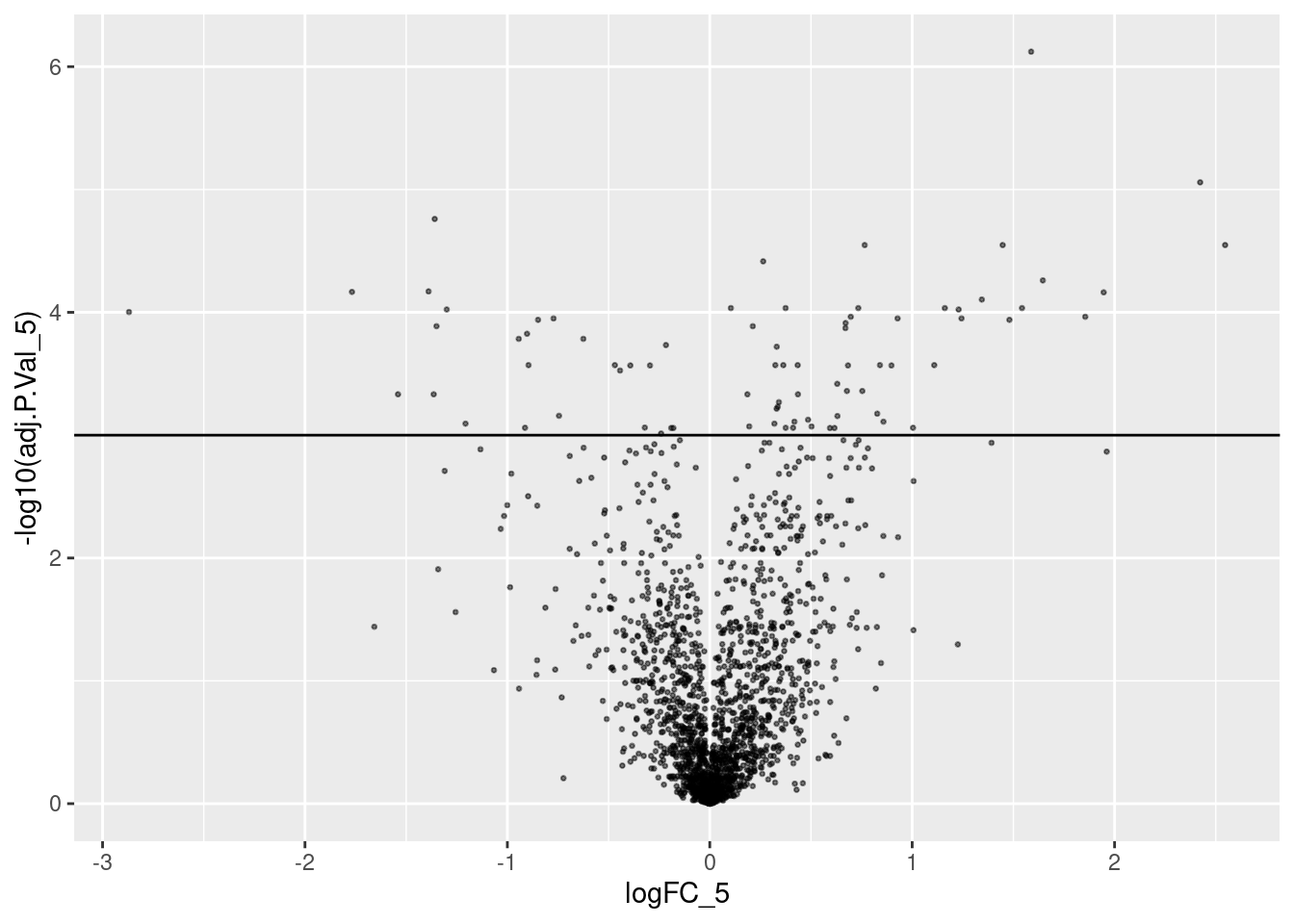
| Version | Author | Date |
|---|---|---|
| bb9a8b6 | Dave Tang | 2025-01-11 |
markers <- nhood_markers$GeneID[nhood_markers$adj.P.Val_5 < 0.01 & nhood_markers$logFC_5 > 0]set.seed(42)
plotNhoodExpressionGroups(embryo_milo, da_results, features=intersect(rownames(embryo_milo), markers[1:10]),
subset.nhoods = da_results$NhoodGroup %in% c('6','5'),
scale=TRUE,
grid.space = "fixed")Warning in plotNhoodExpressionGroups(embryo_milo, da_results, features =
intersect(rownames(embryo_milo), : Nothing in nhoodExpression(x): computing for
requested features...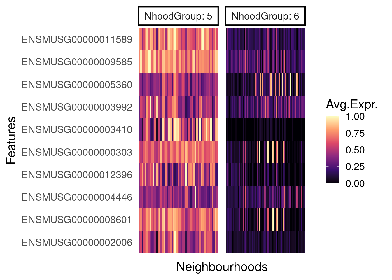
| Version | Author | Date |
|---|---|---|
| bb9a8b6 | Dave Tang | 2025-01-11 |
DGE testing within a group
dge_6 <- testDiffExp(embryo_milo, da_results, design = ~ stage, meta.data = data.frame(colData(embryo_milo)),
                     subset.row = rownames(embryo_milo)[1:5], subset.nhoods=da_results$NhoodGroup=="6")
Warning in fitFDist(var, df1 = df, covariate = covariate): More than half of
residual variances are exactly zero: eBayes unreliabledge_6$`6`
logFC AveExpr t P.Value adj.P.Val
ENSMUSG00000025902 -0.080567087 0.3520449 -2.023978 0.04314914 0.2157457
ENSMUSG00000033845 -0.009033338 2.2775883 -0.209271 0.83426503 1.0000000
ENSMUSG00000051951 0.000000000 0.0000000 0.000000 1.00000000 1.0000000
ENSMUSG00000102343 0.000000000 0.0000000 0.000000 1.00000000 1.0000000
ENSMUSG00000025900 0.000000000 0.0000000 0.000000 1.00000000 1.0000000
B Nhood.Group
ENSMUSG00000025902 -9.440543 6
ENSMUSG00000033845 -11.465446 6
ENSMUSG00000051951 -11.487357 6
ENSMUSG00000102343 -11.487357 6
ENSMUSG00000025900 -11.487357 6
sessionInfo()R version 4.4.1 (2024-06-14)
Platform: x86_64-pc-linux-gnu
Running under: Ubuntu 22.04.5 LTS
Matrix products: default
BLAS: /usr/lib/x86_64-linux-gnu/openblas-pthread/libblas.so.3
LAPACK: /usr/lib/x86_64-linux-gnu/openblas-pthread/libopenblasp-r0.3.20.so; LAPACK version 3.10.0
locale:
[1] LC_CTYPE=en_US.UTF-8 LC_NUMERIC=C
[3] LC_TIME=en_US.UTF-8 LC_COLLATE=en_US.UTF-8
[5] LC_MONETARY=en_US.UTF-8 LC_MESSAGES=en_US.UTF-8
[7] LC_PAPER=en_US.UTF-8 LC_NAME=C
[9] LC_ADDRESS=C LC_TELEPHONE=C
[11] LC_MEASUREMENT=en_US.UTF-8 LC_IDENTIFICATION=C
time zone: Etc/UTC
tzcode source: system (glibc)
attached base packages:
[1] stats4 stats graphics grDevices utils datasets methods
[8] base
other attached packages:
[1] MouseGastrulationData_1.20.0 SpatialExperiment_1.16.0
[3] patchwork_1.3.0 dplyr_1.1.4
[5] scran_1.34.0 scater_1.34.0
[7] ggplot2_3.5.1 scuttle_1.16.0
[9] SingleCellExperiment_1.28.1 SummarizedExperiment_1.36.0
[11] Biobase_2.66.0 GenomicRanges_1.58.0
[13] GenomeInfoDb_1.42.1 IRanges_2.40.1
[15] S4Vectors_0.44.0 BiocGenerics_0.52.0
[17] MatrixGenerics_1.18.0 matrixStats_1.4.1
[19] miloR_2.2.0 edgeR_4.4.1
[21] limma_3.62.1 workflowr_1.7.1
loaded via a namespace (and not attached):
[1] RColorBrewer_1.1-3 rstudioapi_0.17.1 jsonlite_1.8.9
[4] magrittr_2.0.3 ggbeeswarm_0.7.2 magick_2.8.5
[7] farver_2.1.2 rmarkdown_2.28 fs_1.6.4
[10] zlibbioc_1.52.0 vctrs_0.6.5 memoise_2.0.1
[13] htmltools_0.5.8.1 S4Arrays_1.6.0 curl_6.0.1
[16] AnnotationHub_3.14.0 BiocNeighbors_2.0.1 SparseArray_1.6.0
[19] sass_0.4.9 pracma_2.4.4 bslib_0.8.0
[22] cachem_1.1.0 whisker_0.4.1 igraph_2.1.2
[25] mime_0.12 lifecycle_1.0.4 pkgconfig_2.0.3
[28] rsvd_1.0.5 Matrix_1.7-0 R6_2.5.1
[31] fastmap_1.2.0 GenomeInfoDbData_1.2.13 digest_0.6.37
[34] numDeriv_2016.8-1.1 colorspace_2.1-1 AnnotationDbi_1.68.0
[37] ps_1.8.1 rprojroot_2.0.4 dqrng_0.4.1
[40] irlba_2.3.5.1 ExperimentHub_2.14.0 RSQLite_2.3.9
[43] beachmat_2.22.0 labeling_0.4.3 filelock_1.0.3
[46] fansi_1.0.6 httr_1.4.7 polyclip_1.10-7
[49] abind_1.4-8 compiler_4.4.1 bit64_4.5.2
[52] withr_3.0.2 BiocParallel_1.40.0 DBI_1.2.3
[55] viridis_0.6.5 highr_0.11 ggforce_0.4.2
[58] MASS_7.3-60.2 rappdirs_0.3.3 DelayedArray_0.32.0
[61] rjson_0.2.23 bluster_1.16.0 gtools_3.9.5
[64] tools_4.4.1 vipor_0.4.7 beeswarm_0.4.0
[67] httpuv_1.6.15 glue_1.8.0 callr_3.7.6
[70] promises_1.3.0 grid_4.4.1 getPass_0.2-4
[73] cluster_2.1.6 generics_0.1.3 gtable_0.3.6
[76] tidyr_1.3.1 BiocSingular_1.22.0 tidygraph_1.3.1
[79] ScaledMatrix_1.14.0 metapod_1.14.0 utf8_1.2.4
[82] XVector_0.46.0 RcppAnnoy_0.0.22 BiocVersion_3.20.0
[85] ggrepel_0.9.6 pillar_1.9.0 stringr_1.5.1
[88] BumpyMatrix_1.14.0 later_1.3.2 splines_4.4.1
[91] tweenr_2.0.3 BiocFileCache_2.14.0 lattice_0.22-6
[94] FNN_1.1.4.1 bit_4.5.0 tidyselect_1.2.1
[97] locfit_1.5-9.10 Biostrings_2.74.1 knitr_1.48
[100] git2r_0.35.0 gridExtra_2.3 xfun_0.48
[103] graphlayouts_1.2.0 statmod_1.5.0 stringi_1.8.4
[106] UCSC.utils_1.2.0 yaml_2.3.10 evaluate_1.0.1
[109] codetools_0.2-20 ggraph_2.2.1 tibble_3.2.1
[112] BiocManager_1.30.25 cli_3.6.3 uwot_0.2.2
[115] munsell_0.5.1 processx_3.8.4 jquerylib_0.1.4
[118] Rcpp_1.0.13 dbplyr_2.5.0 png_0.1-8
[121] parallel_4.4.1 blob_1.2.4 viridisLite_0.4.2
[124] scales_1.3.0 purrr_1.0.2 crayon_1.5.3
[127] rlang_1.1.4 KEGGREST_1.46.0 cowplot_1.1.3