Step by step Principal Components Analysis in R
2022-10-20
Last updated: 2022-10-20
Checks: 7 0
Knit directory: muse/
This reproducible R Markdown analysis was created with workflowr (version 1.7.0). The Checks tab describes the reproducibility checks that were applied when the results were created. The Past versions tab lists the development history.
Great! Since the R Markdown file has been committed to the Git repository, you know the exact version of the code that produced these results.
Great job! The global environment was empty. Objects defined in the global environment can affect the analysis in your R Markdown file in unknown ways. For reproduciblity it’s best to always run the code in an empty environment.
The command set.seed(20200712) was run prior to running
the code in the R Markdown file. Setting a seed ensures that any results
that rely on randomness, e.g. subsampling or permutations, are
reproducible.
Great job! Recording the operating system, R version, and package versions is critical for reproducibility.
Nice! There were no cached chunks for this analysis, so you can be confident that you successfully produced the results during this run.
Great job! Using relative paths to the files within your workflowr project makes it easier to run your code on other machines.
Great! You are using Git for version control. Tracking code development and connecting the code version to the results is critical for reproducibility.
The results in this page were generated with repository version f9bfcec. See the Past versions tab to see a history of the changes made to the R Markdown and HTML files.
Note that you need to be careful to ensure that all relevant files for
the analysis have been committed to Git prior to generating the results
(you can use wflow_publish or
wflow_git_commit). workflowr only checks the R Markdown
file, but you know if there are other scripts or data files that it
depends on. Below is the status of the Git repository when the results
were generated:
Ignored files:
    Ignored:    .Rhistory
    Ignored:    .Rproj.user/
    Ignored:    r_packages_4.1.2/
    Ignored:    r_packages_4.2.0/

Untracked files:
    Untracked:  analysis/cell_ranger.Rmd
    Untracked:  data/ncrna_NONCODE[v3.0].fasta.tar.gz
    Untracked:  data/ncrna_noncode_v3.fa
Note that any generated files, e.g. HTML, png, CSS, etc., are not included in this status report because it is ok for generated content to have uncommitted changes.
These are the previous versions of the repository in which changes were
made to the R Markdown (analysis/pca.Rmd) and HTML
(docs/pca.html) files. If you’ve configured a remote Git
repository (see ?wflow_git_remote), click on the hyperlinks
in the table below to view the files as they were in that past version.
| File | Version | Author | Date | Message |
|---|---|---|---|---|
| Rmd | f9bfcec | Dave Tang | 2022-10-20 | PCA |
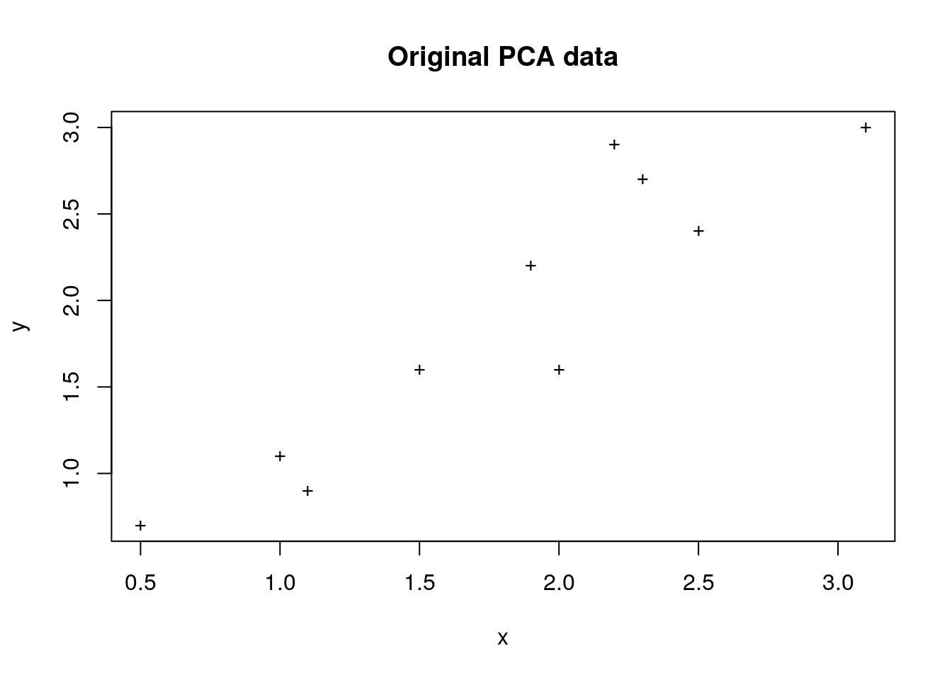
I have always wondered what goes on behind the scenes of a Principal Components Analysis (PCA). I found this extremely useful tutorial (that I have hosted on my server for the sake of prosperity), which explains the key concepts behind the PCA and also shows the step by step calculations. Here, I use R to perform each step of a PCA as per the tutorial.
pca_data <- data.frame(
  x = c(2.5, 0.5, 2.2, 1.9, 3.1, 2.3, 2, 1, 1.5, 1.1),
  y = c(2.4, 0.7, 2.9, 2.2, 3.0, 2.7, 1.6, 1.1, 1.6, 0.9)
)

plot(
  pca_data,
  pch = '+',
  main = "Original PCA data"
)
Next, we need to work out the mean of each dimension and subtract it from each value from the respective dimensions. This is known as standardisation, where the dimensions now have a mean of zero.
pca_data_scaled <- apply(pca_data, 2, function(x) x - mean(x))

plot(
  pca_data_scaled,
  pch = '+',
  main = "Scaled PCA data"
)
The next step is to calculate the covariance matrix. Covariance measures how dimensions vary with respect to each other and the covariance matrix contains all covariance measures between all dimensions.
m <- cov(pca_data_scaled)
m
x y
x 0.6165556 0.6154444
y 0.6154444 0.7165556Next we need to find the eigenvector and eigenvalues of the covariance matrix. An eigenvector is a direction and an eigenvalue is a number that indicates how much variance is in the data in that direction. Note that the eigenvalues calculated here are the same as the tutorial (but in a different order). However, the first eigenvector calculated are negative in the tutorial.
e <- eigen(m)
e
eigen() decomposition
$values
[1] 1.2840277 0.0490834
$vectors
[,1] [,2]
[1,] 0.6778734 -0.7351787
[2,] 0.7351787 0.6778734The largest eigenvalue is the first principal component and the second largest is the second principal component; we multiply the standardised values to the eigenvectors to obtain the principal components.
my_pca <- as.matrix(pca_data_scaled) %*% e$vectors

plot(
  my_pca,
  pch = '+',
  xlab = "PC1",
  ylab = "PC2",
  main = "PCA (manual) plot"
)
Now to perform PCA using the prcomp() function.
pca <- prcomp(pca_data)
summary(pca)
Importance of components:
PC1 PC2
Standard deviation 1.1331 0.22155
Proportion of Variance 0.9632 0.03682
Cumulative Proportion 0.9632 1.00000plot(
pca$x,
pch = 16,
col = 1,
xlab = "PC1",
ylab = "PC2",
main = "PCA (prcomp) plot"
)
points(
my_pca,
pch = 16,
col = 2
)
This post
on Stack Overflow suggests that setting the symmetric
argument is the reason for the difference in the eigenvector signs and
the bottom line is that this does not matter anyway.
eigen(m)eigen() decomposition
$values
[1] 1.2840277 0.0490834
$vectors
[,1] [,2]
[1,] 0.6778734 -0.7351787
[2,] 0.7351787 0.6778734pcaStandard deviations (1, .., p=2):
[1] 1.1331495 0.2215477
Rotation (n x k) = (2 x 2):
PC1 PC2
x -0.6778734 0.7351787
y -0.7351787 -0.6778734But I still can’t replicate the sign from prcomp.
eigen(m, symmetric = TRUE)eigen() decomposition
$values
[1] 1.2840277 0.0490834
$vectors
[,1] [,2]
[1,] 0.6778734 -0.7351787
[2,] 0.7351787 0.6778734eigen(m, symmetric = FALSE)eigen() decomposition
$values
[1] 1.2840277 0.0490834
$vectors
[,1] [,2]
[1,] -0.6778734 -0.7351787
[2,] -0.7351787 0.6778734pcaStandard deviations (1, .., p=2):
[1] 1.1331495 0.2215477
Rotation (n x k) = (2 x 2):
PC1 PC2
x -0.6778734 0.7351787
y -0.7351787 -0.6778734However, the eigenvectors calculated in the tutorial can be
replicated with symmetric = FALSE (but with the larger
eigenvalue displayed last).
tut_eigen <- matrix(c(-0.735178656, -0.677873399, 0.677873399, -0.735178656), nrow = 2, byrow = TRUE)
eigen(m, symmetric = FALSE)
eigen() decomposition
$values
[1] 1.2840277 0.0490834
$vectors
[,1] [,2]
[1,] -0.6778734 -0.7351787
[2,] -0.7351787 0.6778734tut_eigen [,1] [,2]
[1,] -0.7351787 -0.6778734
[2,] 0.6778734 -0.7351787The help page of eigen states that if symmetric is TRUE,
the matrix is assumed to be symmetric (or Hermitian if complex) and only
its lower triangle (diagonal included) is used. Since the covariance
matrix is symmetric, we should really use
symmetric = TRUE.
isSymmetric(m)[1] TRUEFurther reading
sessionInfo()R version 4.2.0 (2022-04-22)
Platform: x86_64-pc-linux-gnu (64-bit)
Running under: Ubuntu 20.04.4 LTS
Matrix products: default
BLAS: /usr/lib/x86_64-linux-gnu/openblas-pthread/libblas.so.3
LAPACK: /usr/lib/x86_64-linux-gnu/openblas-pthread/liblapack.so.3
locale:
[1] LC_CTYPE=en_US.UTF-8 LC_NUMERIC=C
[3] LC_TIME=en_US.UTF-8 LC_COLLATE=en_US.UTF-8
[5] LC_MONETARY=en_US.UTF-8 LC_MESSAGES=en_US.UTF-8
[7] LC_PAPER=en_US.UTF-8 LC_NAME=C
[9] LC_ADDRESS=C LC_TELEPHONE=C
[11] LC_MEASUREMENT=en_US.UTF-8 LC_IDENTIFICATION=C
attached base packages:
[1] stats graphics grDevices utils datasets methods base
other attached packages:
[1] forcats_0.5.1 stringr_1.4.0 dplyr_1.0.9 purrr_0.3.4
[5] readr_2.1.2 tidyr_1.2.0 tibble_3.1.8 ggplot2_3.3.6
[9] tidyverse_1.3.1 workflowr_1.7.0
loaded via a namespace (and not attached):
[1] Rcpp_1.0.8.3 lubridate_1.8.0 getPass_0.2-2 ps_1.7.0
[5] assertthat_0.2.1 rprojroot_2.0.3 digest_0.6.29 utf8_1.2.2
[9] R6_2.5.1 cellranger_1.1.0 backports_1.4.1 reprex_2.0.1
[13] evaluate_0.15 highr_0.9 httr_1.4.3 pillar_1.8.1
[17] rlang_1.0.4 readxl_1.4.0 rstudioapi_0.13 whisker_0.4
[21] callr_3.7.0 jquerylib_0.1.4 rmarkdown_2.14 munsell_0.5.0
[25] broom_0.8.0 compiler_4.2.0 httpuv_1.6.5 modelr_0.1.8
[29] xfun_0.31 pkgconfig_2.0.3 htmltools_0.5.2 tidyselect_1.1.2
[33] fansi_1.0.3 crayon_1.5.1 tzdb_0.3.0 dbplyr_2.1.1
[37] withr_2.5.0 later_1.3.0 grid_4.2.0 jsonlite_1.8.0
[41] gtable_0.3.0 lifecycle_1.0.1 DBI_1.1.2 git2r_0.30.1
[45] magrittr_2.0.3 scales_1.2.0 cli_3.3.0 stringi_1.7.6
[49] fs_1.5.2 promises_1.2.0.1 xml2_1.3.3 bslib_0.3.1
[53] ellipsis_0.3.2 generics_0.1.3 vctrs_0.4.1 tools_4.2.0
[57] glue_1.6.2 hms_1.1.2 processx_3.5.3 fastmap_1.1.0
[61] yaml_2.3.5 colorspace_2.0-3 rvest_1.0.2 knitr_1.39
[65] haven_2.5.0 sass_0.4.1