Quantile normalisation in R
2023-10-12
Last updated: 2023-10-12
Checks: 7 0
Knit directory: muse/
This reproducible R Markdown analysis was created with workflowr (version 1.7.0). The Checks tab describes the reproducibility checks that were applied when the results were created. The Past versions tab lists the development history.
Great! Since the R Markdown file has been committed to the Git repository, you know the exact version of the code that produced these results.
Great job! The global environment was empty. Objects defined in the global environment can affect the analysis in your R Markdown file in unknown ways. For reproduciblity it’s best to always run the code in an empty environment.
The command set.seed(20200712) was run prior to running
the code in the R Markdown file. Setting a seed ensures that any results
that rely on randomness, e.g. subsampling or permutations, are
reproducible.
Great job! Recording the operating system, R version, and package versions is critical for reproducibility.
Nice! There were no cached chunks for this analysis, so you can be confident that you successfully produced the results during this run.
Great job! Using relative paths to the files within your workflowr project makes it easier to run your code on other machines.
Great! You are using Git for version control. Tracking code development and connecting the code version to the results is critical for reproducibility.
The results in this page were generated with repository version 848ea4b. See the Past versions tab to see a history of the changes made to the R Markdown and HTML files.
Note that you need to be careful to ensure that all relevant files for
the analysis have been committed to Git prior to generating the results
(you can use wflow_publish or
wflow_git_commit). workflowr only checks the R Markdown
file, but you know if there are other scripts or data files that it
depends on. Below is the status of the Git repository when the results
were generated:
Ignored files:
    Ignored:    .Rhistory
    Ignored:    .Rproj.user/
    Ignored:    r_packages_4.3.0/
    Ignored:    r_packages_4.3.1/

Untracked files:
    Untracked:  analysis/cell_ranger.Rmd
    Untracked:  analysis/complex_heatmap.Rmd
    Untracked:  analysis/sleuth.Rmd
    Untracked:  analysis/tss_xgboost.Rmd
    Untracked:  code/multiz100way/
    Untracked:  data/HG00702_SH089_CHSTrio.chr1.vcf.gz
    Untracked:  data/HG00702_SH089_CHSTrio.chr1.vcf.gz.tbi
    Untracked:  data/ncrna_NONCODE[v3.0].fasta.tar.gz
    Untracked:  data/ncrna_noncode_v3.fa
    Untracked:  data/netmhciipan.out.gz
    Untracked:  data/test
    Untracked:  export/davetang039sblog.WordPress.2023-06-30.xml
    Untracked:  export/output/
    Untracked:  women.json

Unstaged changes:
    Modified:   analysis/graph.Rmd
    Modified:   analysis/tissue.Rmd
Note that any generated files, e.g. HTML, png, CSS, etc., are not included in this status report because it is ok for generated content to have uncommitted changes.
These are the previous versions of the repository in which changes were
made to the R Markdown (analysis/qn.Rmd) and HTML
(docs/qn.html) files. If you’ve configured a remote Git
repository (see ?wflow_git_remote), click on the hyperlinks
in the table below to view the files as they were in that past version.
| File | Version | Author | Date | Message |
|---|---|---|---|---|
| Rmd | 848ea4b | Dave Tang | 2023-10-12 | Use median for average |
| html | 78011d1 | Dave Tang | 2023-10-12 | Build site. |
| Rmd | 4a7d5e8 | Dave Tang | 2023-10-12 | One more example |
| html | 2e70b5b | Dave Tang | 2023-10-12 | Build site. |
| Rmd | dc2b970 | Dave Tang | 2023-10-12 | Fix title and summary |
| html | f715b16 | Dave Tang | 2023-10-12 | Build site. |
| Rmd | 1ede478 | Dave Tang | 2023-10-12 | Quantile normalisation |
From Wikipedia:
In statistics, quantile normalization is a technique for making two distributions identical in statistical properties. To quantile normalize two or more distributions to each other, without a reference distribution, sort as before, then set to the average (usually, arithmetical mean) of the distributions. So the highest value in all cases becomes the mean of the highest values, the second highest value becomes the mean of the second highest values, and so on.
Wikipedia example
In this section, we will follow the Wikipedia example. First we will create the data set; we will use a list to store everything. The raw data contains four genes (A to D) and three samples (x to z).
eg1 <- list()

eg1$raw <- data.frame(
  x=c(5,2,3,4),
  y=c(4,1,4,2),
  z=c(3,4,6,8)
)

rownames(eg1$raw) <- toupper(letters[1:4])

eg1$raw
x y z
A 5 4 3
B 2 1 4
C 3 4 6
D 4 2 8The first step is to determine the gene ranks per sample; the lowest expressed gene will be the smallest number and the highest expressed gene will be largest number. This could be from 1 to 4 but if two genes have the same expression, i.e., tied, then the largest number won’t be 4.
eg1$rank <- apply(eg1$raw, 2, rank, ties.method="min")
eg1$rank
x y z
A 4 3 1
B 1 1 2
C 2 3 3
D 3 2 4Next, we sort the genes by their expression per sample. The lowest expressed gene will be on the top and the highest expressed gene will be on the bottom.
eg1$sorted <- data.frame(apply(eg1$raw, 2, sort))
eg1$sorted
x y z
1 2 1 3
2 3 2 4
3 4 4 6
4 5 4 8We will use the sorted gene expression matrix to calculate row means.
eg1$mean <- rowMeans(eg1$sorted)
eg1$mean
[1] 2.000000 3.000000 4.666667 5.666667Finally, we will use the row means as the normalised values for each gene. Since every sample now uses the same set of means for the expression values, every sample will have the same statistical properties.
We will use the raw ranking to determine which mean value to use. For example, if gene A was the most highly expressed gene in sample x, then it will get the highest mean value. The code above simply uses the gene ranks as the index to the means.
eg1$norm <- apply(eg1$rank, 2, function(x) eg1$mean[x])
rownames(eg1$norm) <- toupper(letters[1:4])
eg1$norm
x y z
A 5.666667 4.666667 2.000000
B 2.000000 2.000000 3.000000
C 3.000000 4.666667 4.666667
D 4.666667 3.000000 5.666667We can combine all the code above (with some additional code for
normalising with an average rank method) and save it into a
quantile_normalisation function.
quantile_normalisation <- function(x, ties = "min"){
  my_list <- list()
  my_list$raw <- x
  my_list$rank <- apply(my_list$raw, 2, rank, ties.method=ties)
  my_list$sorted <- data.frame(apply(my_list$raw, 2, sort))
  my_list$mean <- rowMeans(my_list$sorted)
  # my dumb implementation of using average
  if(ties == "average"){
     my_list$norm <- apply(my_list$raw, 2, function(v){
      my_min <- rank(v, ties.method = "min")
      my_max <- rank(v, ties.method = "max")
      sapply(seq_along(my_min), function(i){
        m <- my_list$mean[my_min[i]:my_max[i]]
        median(m)
      })
    })
  } else {
    my_list$norm <- apply(my_list$rank, 2, function(i) my_list$mean[i])
  }
  rownames(my_list$norm) <- rownames(my_list$raw)
  return(my_list)
}

my_df <- data.frame(
  one=c(5,2,3,4),
  two=c(4,1,4,2),
  three=c(3,4,6,8)
)
rownames(my_df) <- toupper(letters[1:4])

quantile_normalisation(my_df)$norm
one two three
A 5.666667 4.666667 2.000000
B 2.000000 2.000000 3.000000
C 3.000000 4.666667 4.666667
D 4.666667 3.000000 5.666667PH525x example
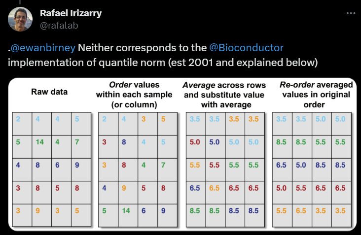
The data used for this example was from edX course called PH525x but it does not seem to be available anymore; it is probably called something else now. I’ll use this example because the process of quantile normalisation is nicely summarised in the figure below (the figure was from the bird app but I don’t want to link to it):
eg2 <- list()
eg2$raw <- matrix(
  data = c(2,4,4,5,5,14,4,7,4,8,6,9,3,8,5,8,3,9,3,5),
  nrow = 5,
  byrow = TRUE,
  dimnames = list(toupper(LETTERS[1:5]), letters[23:26])
)

eg2$raw
w x y z
A 2 4 4 5
B 5 14 4 7
C 4 8 6 9
D 3 8 5 8
E 3 9 3 5Order values within each sample (or column).
eg2$rank <- apply(eg2$raw, 2, rank, ties.method="min")
eg2$sorted <- apply(eg2$raw, 2, sort)
eg2$sorted
w x y z
[1,] 2 4 3 5
[2,] 3 8 4 5
[3,] 3 8 4 7
[4,] 4 9 5 8
[5,] 5 14 6 9Average across rows.
eg2$mean <- rowMeans(eg2$sorted)
eg2$mean
[1] 3.5 5.0 5.5 6.5 8.5Re-order averaged values in original order.
eg2$norm <- apply(eg2$rank, 2, function(i) eg2$mean[i])
eg2$norm
w x y z
[1,] 3.5 3.5 5.0 3.5
[2,] 8.5 8.5 5.0 5.5
[3,] 6.5 5.0 8.5 8.5
[4,] 5.0 5.0 6.5 6.5
[5,] 5.0 6.5 3.5 3.5Notice that my values are slightly different from those in the
figure; this is because I used the minimum value for rank()
when there is a tie.
In the rank() function, there are several methods for
dealing with ties:
- “average”
- “first”
- “last”
- “random”
- “max”
- “min”
Here’s the documentation for the different methods.
If all components are different (and no NAs), the ranks are well defined, with values in seq_along(x). With some values equal (called “ties”), the argument ties.method determines the result at the corresponding indices. The “first” method results in a permutation with increasing values at each index set of ties, and analogously “last” with decreasing values. The “random” method puts these in random order whereas the default, “average”, replaces them by their mean, and “max” and “min” replaces them by their maximum and minimum respectively, the latter being the typical sports ranking.
The values in the PH525x example were calculated using a “first”
approach. We can specify this in our quantile_normalisation
function, and now we have the same normalised values.
quantile_normalisation(eg2$raw, ties = "first")$norm w x y z
A 3.5 3.5 5.0 3.5
B 8.5 8.5 5.5 5.5
C 6.5 5.0 8.5 8.5
D 5.0 5.5 6.5 6.5
E 5.5 6.5 3.5 5.0But those with a keen eye will notice that this is also different
from the figure. This is to do with the ordering for the expression
values that are tied and this is not consistent in the figure. If we go
with a “first” approach then the ordering should be from gene A to E. If
gene A and E are tied, then gene A will be ranked ahead of E because it
comes first. If gene C and D are tied, then gene C is ranked ahead of D.
This is what is performed with the rank function.
eg2$raw w x y z
A 2 4 4 5
B 5 14 4 7
C 4 8 6 9
D 3 8 5 8
E 3 9 3 5quantile_normalisation(eg2$raw, ties = "first")$rank w x y z
A 1 1 2 1
B 5 5 3 3
C 4 2 5 5
D 2 3 4 4
E 3 4 1 2In the figure, gene D and E in sample w are ranked in a first manner and get the mean values in this order; so is gene C and D in sample x, and gene B and C in sample y. But this is not the case for gene A and E in sample z; gene A should get the 3.5 value and gene E should get the 5.0 value, if we want to be consistent.
Bioconductor
The preprocessCore package on Bioconductor already has a
function for quantile normalisation called
normalize.quantiles. Install the package, if necessary.
Note that if I try to install the package the usual
way, I get the following error:
Error in normalize.quantiles(mat) :
  ERROR; return code from pthread_create() is 22
This is a known issue
and I can use the function if I install preprocessCore as
per these
instructions.
if (!require("BiocManager", quietly = TRUE))
    install.packages("BiocManager")

BiocManager::install("preprocessCore", configure.args = c(preprocessCore = "--disable-threading"), force= TRUE, update=TRUE, type = "source")
The normalize.quantiles function takes a matrix as
input.
library(preprocessCore)

normalize.quantiles(eg2$raw)
[,1] [,2] [,3] [,4]
[1,] 3.50 3.50 5.25 4.25
[2,] 8.50 8.50 5.25 5.50
[3,] 6.50 5.25 8.50 8.50
[4,] 5.25 5.25 6.50 6.50
[5,] 5.25 6.50 3.50 4.25The normalize.quantiles function uses the average method
for ties, which we can reproduce with our function.
quantile_normalisation(eg2$raw, ties = "average")$norm w x y z
A 3.50 3.50 5.25 4.25
B 8.50 8.50 5.25 5.50
C 6.50 5.25 8.50 8.50
D 5.25 5.25 6.50 6.50
E 5.25 6.50 3.50 4.25In this example, I have genes tied by different number of times.
eg3 <- matrix(
  data = c(
    2,4,4,9,
    5,14,4,9,
    2,8,4,9,
    3,8,4,9,
    3,8,3,9),
  nrow = 5,
  byrow = TRUE,
  dimnames = list(toupper(LETTERS[1:5]), letters[23:26])
)

eg3
w x y z
A 2 4 4 9
B 5 14 4 9
C 2 8 4 9
D 3 8 4 9
E 3 8 3 9Again, we can reproduce the values with our function.
normalize.quantiles(eg3) [,1] [,2] [,3] [,4]
[1,] 5.125 4.5 6.0 6
[2,] 8.000 8.0 6.0 6
[3,] 5.125 6.0 6.0 6
[4,] 6.000 6.0 6.0 6
[5,] 6.000 6.0 4.5 6quantile_normalisation(eg3, ties = "average")$norm w x y z
A 5.125 4.5 6.0 6
B 8.000 8.0 6.0 6
C 5.125 6.0 6.0 6
D 6.000 6.0 6.0 6
E 6.000 6.0 4.5 6Summary
Quantile normalisation was a normalisation method developed for microarrays but is commonly used in RNA-seq as well. It uses ranked expression values, so it is robust against outliers. In order to make every sample have the same statistical properties, mean expression values are calculated using the ranked expression values from every sample. This calculation will result in a (ranked) mean expression value for every gene. These mean expression values are then used in every sample based on the ranking of the raw values. Therefore, the statistical properties, such as the mean and variance, of every sample is the same (and just the ordering is different).
The normalisation method is easy to implement but requires more work
if you want to optimise the code for better performance. There are many
different implementations of the method because there are different ways
to rank items that are tied. The Wikipedia example uses a minimum
approach; the example by Rafael Irizarry uses a first approach; and the
preprocessCore package uses an average approach. I don’t
think changing the way for how ties are treated will significantly
impact the results. To me, the average approach seems like a very
reasonable way to deal with ties.
If you want to perform quantile normalisation, I suggest that you use
the normalize.quantiles function from the
preprocessCore package. If you use it for your work, you
should cite:
I do not suggest using my quantile_normalisation
function except for learning purposes.
sessionInfo()R version 4.3.1 (2023-06-16)
Platform: x86_64-pc-linux-gnu (64-bit)
Running under: Ubuntu 22.04.3 LTS
Matrix products: default
BLAS: /usr/lib/x86_64-linux-gnu/openblas-pthread/libblas.so.3
LAPACK: /usr/lib/x86_64-linux-gnu/openblas-pthread/libopenblasp-r0.3.20.so; LAPACK version 3.10.0
locale:
[1] LC_CTYPE=en_US.UTF-8 LC_NUMERIC=C
[3] LC_TIME=en_US.UTF-8 LC_COLLATE=en_US.UTF-8
[5] LC_MONETARY=en_US.UTF-8 LC_MESSAGES=en_US.UTF-8
[7] LC_PAPER=en_US.UTF-8 LC_NAME=C
[9] LC_ADDRESS=C LC_TELEPHONE=C
[11] LC_MEASUREMENT=en_US.UTF-8 LC_IDENTIFICATION=C
time zone: Etc/UTC
tzcode source: system (glibc)
attached base packages:
[1] stats graphics grDevices utils datasets methods base
other attached packages:
[1] preprocessCore_1.62.1 workflowr_1.7.0
loaded via a namespace (and not attached):
[1] jsonlite_1.8.7 compiler_4.3.1 promises_1.2.1 Rcpp_1.0.11
[5] stringr_1.5.0 git2r_0.32.0 callr_3.7.3 later_1.3.1
[9] jquerylib_0.1.4 yaml_2.3.7 fastmap_1.1.1 R6_2.5.1
[13] knitr_1.43 tibble_3.2.1 rprojroot_2.0.3 bslib_0.5.0
[17] pillar_1.9.0 rlang_1.1.1 utf8_1.2.3 cachem_1.0.8
[21] stringi_1.7.12 httpuv_1.6.11 xfun_0.40 getPass_0.2-2
[25] fs_1.6.3 sass_0.4.7 cli_3.6.1 magrittr_2.0.3
[29] ps_1.7.5 digest_0.6.33 processx_3.8.2 rstudioapi_0.15.0
[33] lifecycle_1.0.3 vctrs_0.6.3 evaluate_0.21 glue_1.6.2
[37] whisker_0.4.1 fansi_1.0.4 rmarkdown_2.23 httr_1.4.6
[41] tools_4.3.1 pkgconfig_2.0.3 htmltools_0.5.6