Rand Index versus the Adjusted Rand Index
2024-06-19
Last updated: 2024-06-19
Checks: 7 0
Knit directory: muse/
This reproducible R Markdown analysis was created with workflowr (version 1.7.1). The Checks tab describes the reproducibility checks that were applied when the results were created. The Past versions tab lists the development history.
Great! Since the R Markdown file has been committed to the Git repository, you know the exact version of the code that produced these results.
Great job! The global environment was empty. Objects defined in the global environment can affect the analysis in your R Markdown file in unknown ways. For reproduciblity it’s best to always run the code in an empty environment.
The command set.seed(20200712) was run prior to running
the code in the R Markdown file. Setting a seed ensures that any results
that rely on randomness, e.g. subsampling or permutations, are
reproducible.
Great job! Recording the operating system, R version, and package versions is critical for reproducibility.
Nice! There were no cached chunks for this analysis, so you can be confident that you successfully produced the results during this run.
Great job! Using relative paths to the files within your workflowr project makes it easier to run your code on other machines.
Great! You are using Git for version control. Tracking code development and connecting the code version to the results is critical for reproducibility.
The results in this page were generated with repository version 19fb6e6. See the Past versions tab to see a history of the changes made to the R Markdown and HTML files.
Note that you need to be careful to ensure that all relevant files for
the analysis have been committed to Git prior to generating the results
(you can use wflow_publish or
wflow_git_commit). workflowr only checks the R Markdown
file, but you know if there are other scripts or data files that it
depends on. Below is the status of the Git repository when the results
were generated:
Ignored files:
    Ignored:    .Rhistory
    Ignored:    .Rproj.user/
    Ignored:    r_packages_4.3.3/
    Ignored:    r_packages_4.4.0/
Note that any generated files, e.g. HTML, png, CSS, etc., are not included in this status report because it is ok for generated content to have uncommitted changes.
These are the previous versions of the repository in which changes were
made to the R Markdown
(analysis/rand_index_vs_adjusted.Rmd) and HTML
(docs/rand_index_vs_adjusted.html) files. If you’ve
configured a remote Git repository (see ?wflow_git_remote),
click on the hyperlinks in the table below to view the files as they
were in that past version.
| File | Version | Author | Date | Message |
|---|---|---|---|---|
| Rmd | 19fb6e6 | Dave Tang | 2024-06-19 | Rand Index versus Adjusted Rand Index |
I wrote about the Rand Index (RI) and the Adjusted Rand Index (ARI) but how do we interpret the indices and how are they different?
As a quick recap, the RI is:
\[ RI = \frac{a + b}{ { {n}\choose{2} } } \]
where \(a\) and \(b\) are the number of times a pair of
elements were clustered concordantly in two different sets, like
clustering results. I wrote some code (based on
fossil::rand.index) that calculates the RI, as well as
returning values for \(a\), \(b\), and \(n\choose{2}\).
rand_index <- function(group1, group2){
  x <- abs(sapply(group1, \(x) x - group1))
  x[x > 1] <- 1
  y <- abs(sapply(group2, \(x) x - group2))
  y[y > 1] <- 1
  i <- x[upper.tri(x)] == y[upper.tri(y)]
  a <- sum(x[upper.tri(x)][i] == 0)
  b <- sum(x[upper.tri(x)][i] == 1)
  bc <- choose(length(group1), 2)
  ri <- (a + b) / bc
  list(a = a, b = b, denom = bc, index = ri)
}
I’ll use the example from my previous post, where I compared a set of known labels with results from k-means clustering:
set.seed(1984)
true_label <- as.numeric(iris$Species)
my_kmeans <- kmeans(x = iris[,-5], centers = 3)

rand_index(true_label, my_kmeans$cluster)
$a
[1] 3075
$b
[1] 6756
$denom
[1] 11175
$index
[1] 0.8797315Since the RI ranges from 0 to 1, an index of 0.8797315 implies that the two sets are similar. But how does this compare with a random set? The ARI takes randomness into account and is defined as:
\[ ARI = \frac{ \sum_{ij} { {n_{ij}}\choose{2} } - [ \sum_{i} { {a_{i}}\choose{2} } \sum_{j} { {b_{j}}\choose{2} } ] / { {n}\choose{2} } } { \frac{1}{2} [ \sum_{i} { a_{i}\choose{2} } + \sum_{j} { {b_{j}}\choose{2} } ] - [ \sum_{i} { {a_{i}}\choose{2} } \sum_{j} { {b_{j}}\choose{2} } ] / { {n}\choose{2} } } \]
See my previous post for an explanation of the ARI. I wrote some code below that will return the ARI, as well as each part of the ARI formula.
adjusted_rand_index <- function(x, y){
  my_table <- table(x, y)
  my_choose <- \(x) choose(x, 2)
  n_ij <- sum(sapply(my_table, my_choose))
  a_i <- sum(sapply(rowSums(my_table), my_choose))
  b_j <- sum(sapply(colSums(my_table), my_choose))
  c <- my_choose(length(x))
  e <- a_i*b_j/c
  ari <- (n_ij - e) / (1/2*(a_i+b_j) - e)
  list(n_ij = n_ij, a_i = a_i, b_j = b_j, c = c, e = e, index = ari)
}
Here’s the ARI for the previous example.
adjusted_rand_index(true_label, my_kmeans$cluster)$n_ij
[1] 3075
$a_i
[1] 3675
$b_j
[1] 3819
$c
[1] 11175
$e
[1] 1255.913
$index
[1] 0.7302383The ARI (0.7302383) is slightly lower than the RI (0.8797315). Now let’s calculate the RI and ARI between the known labels and a random set.
set.seed(1984)
my_random <- sample(x = true_label, size = length(true_label))

rand_index(true_label, my_random)
$a
[1] 1207
$b
[1] 5032
$denom
[1] 11175
$index
[1] 0.5582998adjusted_rand_index(true_label, my_random)$index[1] -0.0006312925Even with a random set, there is a lot of agreement with the known labels (6239/11175). The ARI provides an index that is close to 0 because it takes into account the chance of overlap. In addition, note that the ARI is a negative value indicating that the amount of overlap is less than expected.
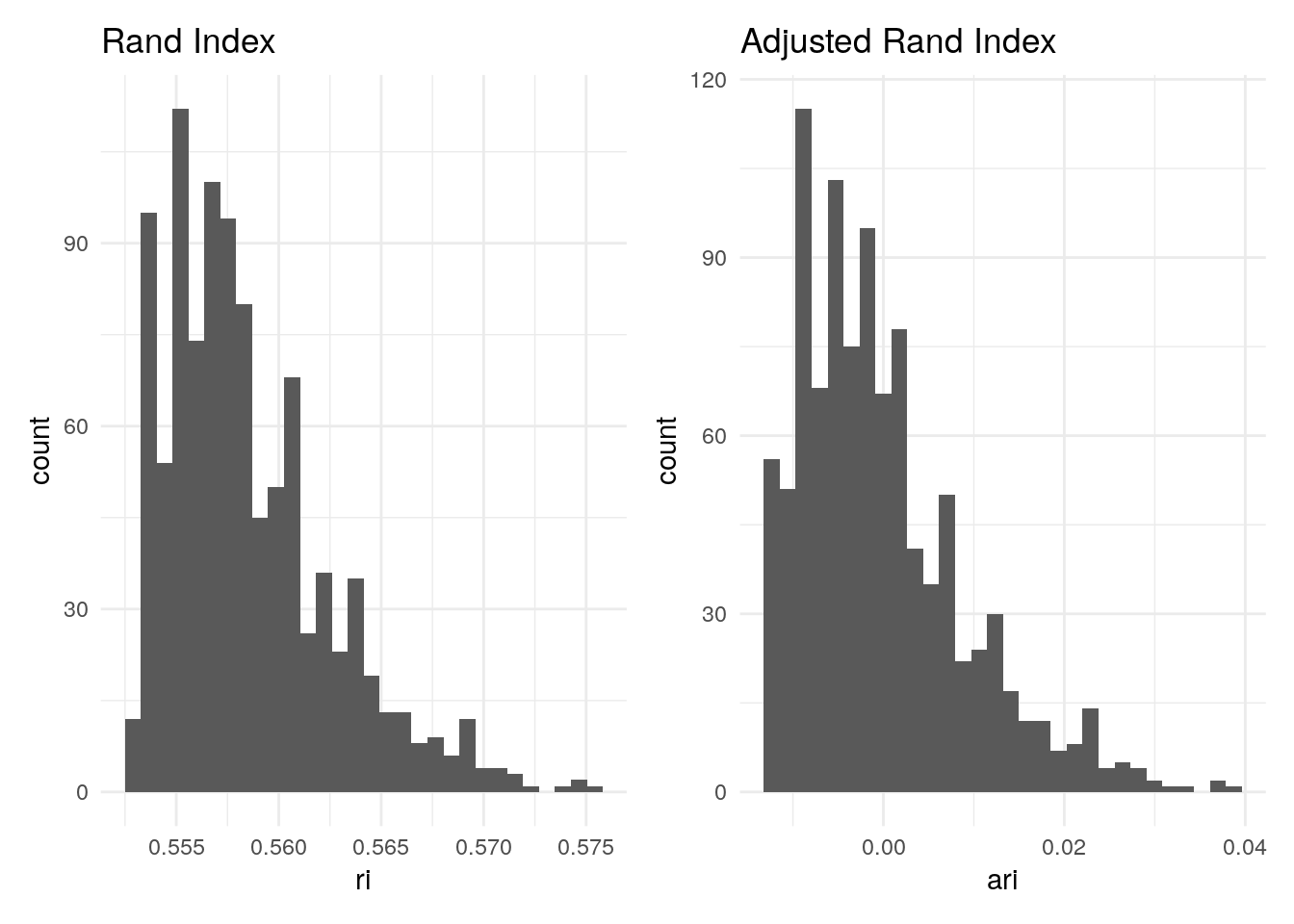
Let’s calculate the RI and ARI for 1,000 randomly sets generated from the known labels of the iris dataset to get a distribution of the indices.
n <- 1000

random_clusters <- purrr::map(1:n, \(x){
  set.seed(x)
  sample(true_label, length(true_label))
})

my_ri <- purrr::map_dbl(random_clusters, \(x) rand_index(true_label, x)$index)
my_ari <- purrr::map_dbl(random_clusters, \(x) adjusted_rand_index(true_label, x)$index)

library(ggplot2)
library(patchwork)

df <- data.frame(ri = my_ri, ari = my_ari)
theme_set(theme_minimal())
ri_plot <- ggplot(df, aes(ri)) + geom_histogram(bins = 30) + ggtitle("Rand Index")
ari_plot <- ggplot(df, aes(ari)) + geom_histogram(bins = 30) + ggtitle("Adjusted Rand Index")
ri_plot + ari_plot
Note that the RI and ARI have a very similar distribution; only the scale on the x-axis differs. In addition, note that the ARI distribution is centred around zero.
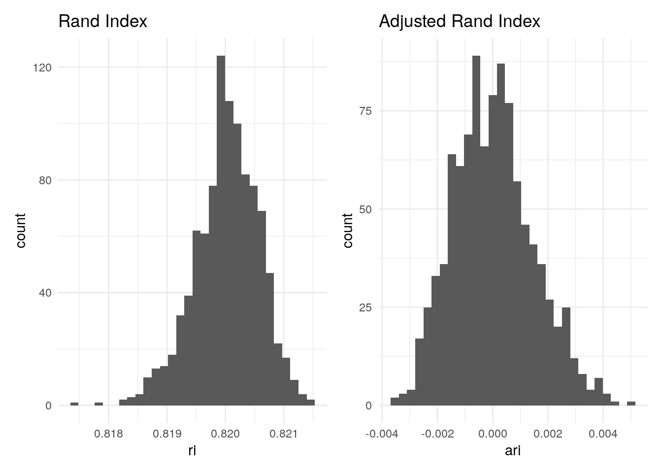
I’ll perform another 1,000 calculations on random sets but this time using larger sets (1,000) and more clusters (10).
n <- 1000

random_clusters_1 <- purrr::map(1:n, \(x){
  set.seed(x)
  sample(1:10, 1000, replace = TRUE)
})

random_clusters_2 <- purrr::map(1:n, \(x){
  set.seed(10000 + x)
  sample(1:10, 1000, replace = TRUE)
})

my_ri <- purrr::map2_dbl(random_clusters_1, random_clusters_2, \(x, y) rand_index(x, y)$index)
my_ari <- purrr::map2_dbl(random_clusters_1, random_clusters_2, \(x, y) adjusted_rand_index(x, y)$index)

df <- data.frame(ri = my_ri, ari = my_ari)
ri_plot <- ggplot(df, aes(ri)) + geom_histogram(bins = 30) + ggtitle("Rand Index")
ari_plot <- ggplot(df, aes(ari)) + geom_histogram(bins = 30) + ggtitle("Adjusted Rand Index")
ri_plot + ari_plot
High RI but low ARI
How do two random sets have a RI that is close to 1? The reason is
due to the number of clusters. When there are a lot of clusters, there’s
a higher chance that a pair of items in both sets are in different
clusters. This is still counted as a concordant event in the RI. If we
run rand_index() we will see that there’s a large
discrepancy between \(a\) and \(b\).
set.seed(1)
x <- sample(1:10, 1000, replace = TRUE)
set.seed(2)
y <- sample(1:10, 1000, replace = TRUE)

rand_index(x, y)
$a
[1] 4953
$b
[1] 404747
$denom
[1] 499500
$index
[1] 0.8202202The ARI on the other hand considers all cluster pairs in contrast to the RI, which only considers whether a pair of elements are in the same cluster or in different clusters.
adjusted_rand_index(x, y)$n_ij
[1] 4953
$a_i
[1] 49844
$b_j
[1] 49862
$c
[1] 499500
$e
[1] 4975.619
$index
[1] -0.0005040106The ARI is based on this contingency table
table(x, y) y
x 1 2 3 4 5 6 7 8 9 10
1 11 7 10 7 11 7 8 13 13 8
2 7 9 6 11 9 9 6 10 8 6
3 12 5 6 14 5 10 9 11 10 14
4 7 8 11 8 10 8 13 14 9 15
5 8 7 14 14 9 14 10 10 12 7
6 7 11 9 12 13 14 11 7 8 7
7 12 11 10 6 7 15 13 16 11 8
8 3 11 6 17 17 13 10 3 6 9
9 12 10 10 16 11 8 9 10 14 8
10 7 14 8 9 12 13 13 10 10 13Conclusion: use the ARI.
sessionInfo()R version 4.4.0 (2024-04-24)
Platform: x86_64-pc-linux-gnu
Running under: Ubuntu 22.04.4 LTS
Matrix products: default
BLAS: /usr/lib/x86_64-linux-gnu/openblas-pthread/libblas.so.3
LAPACK: /usr/lib/x86_64-linux-gnu/openblas-pthread/libopenblasp-r0.3.20.so; LAPACK version 3.10.0
locale:
[1] LC_CTYPE=en_US.UTF-8 LC_NUMERIC=C
[3] LC_TIME=en_US.UTF-8 LC_COLLATE=en_US.UTF-8
[5] LC_MONETARY=en_US.UTF-8 LC_MESSAGES=en_US.UTF-8
[7] LC_PAPER=en_US.UTF-8 LC_NAME=C
[9] LC_ADDRESS=C LC_TELEPHONE=C
[11] LC_MEASUREMENT=en_US.UTF-8 LC_IDENTIFICATION=C
time zone: Etc/UTC
tzcode source: system (glibc)
attached base packages:
[1] stats graphics grDevices utils datasets methods base
other attached packages:
[1] patchwork_1.2.0 lubridate_1.9.3 forcats_1.0.0 stringr_1.5.1
[5] dplyr_1.1.4 purrr_1.0.2 readr_2.1.5 tidyr_1.3.1
[9] tibble_3.2.1 ggplot2_3.5.1 tidyverse_2.0.0 workflowr_1.7.1
loaded via a namespace (and not attached):
[1] sass_0.4.9 utf8_1.2.4 generics_0.1.3 stringi_1.8.4
[5] hms_1.1.3 digest_0.6.35 magrittr_2.0.3 timechange_0.3.0
[9] evaluate_0.23 grid_4.4.0 fastmap_1.2.0 rprojroot_2.0.4
[13] jsonlite_1.8.8 processx_3.8.4 whisker_0.4.1 ps_1.7.6
[17] promises_1.3.0 httr_1.4.7 fansi_1.0.6 scales_1.3.0
[21] jquerylib_0.1.4 cli_3.6.2 rlang_1.1.3 munsell_0.5.1
[25] withr_3.0.0 cachem_1.1.0 yaml_2.3.8 tools_4.4.0
[29] tzdb_0.4.0 colorspace_2.1-0 httpuv_1.6.15 vctrs_0.6.5
[33] R6_2.5.1 lifecycle_1.0.4 git2r_0.33.0 fs_1.6.4
[37] pkgconfig_2.0.3 callr_3.7.6 pillar_1.9.0 bslib_0.7.0
[41] later_1.3.2 gtable_0.3.5 glue_1.7.0 Rcpp_1.0.12
[45] highr_0.10 xfun_0.44 tidyselect_1.2.1 rstudioapi_0.16.0
[49] knitr_1.46 farver_2.1.2 htmltools_0.5.8.1 labeling_0.4.3
[53] rmarkdown_2.27 compiler_4.4.0 getPass_0.2-4