The tidyr pivot_longer and pivot_wider functions using base R
2023-07-26
Last updated: 2023-07-26
Checks: 7 0
Knit directory: muse/
This reproducible R Markdown analysis was created with workflowr (version 1.7.0). The Checks tab describes the reproducibility checks that were applied when the results were created. The Past versions tab lists the development history.
Great! Since the R Markdown file has been committed to the Git repository, you know the exact version of the code that produced these results.
Great job! The global environment was empty. Objects defined in the global environment can affect the analysis in your R Markdown file in unknown ways. For reproduciblity it’s best to always run the code in an empty environment.
The command set.seed(20200712) was run prior to running
the code in the R Markdown file. Setting a seed ensures that any results
that rely on randomness, e.g. subsampling or permutations, are
reproducible.
Great job! Recording the operating system, R version, and package versions is critical for reproducibility.
Nice! There were no cached chunks for this analysis, so you can be confident that you successfully produced the results during this run.
Great job! Using relative paths to the files within your workflowr project makes it easier to run your code on other machines.
Great! You are using Git for version control. Tracking code development and connecting the code version to the results is critical for reproducibility.
The results in this page were generated with repository version 23b5720. See the Past versions tab to see a history of the changes made to the R Markdown and HTML files.
Note that you need to be careful to ensure that all relevant files for
the analysis have been committed to Git prior to generating the results
(you can use wflow_publish or
wflow_git_commit). workflowr only checks the R Markdown
file, but you know if there are other scripts or data files that it
depends on. Below is the status of the Git repository when the results
were generated:
Ignored files:
    Ignored:    .Rhistory
    Ignored:    .Rproj.user/
    Ignored:    r_packages_4.3.0/

Untracked files:
    Untracked:  analysis/cell_ranger.Rmd
    Untracked:  analysis/tss_xgboost.Rmd
    Untracked:  code/multiz100way/
    Untracked:  data/HG00702_SH089_CHSTrio.chr1.vcf.gz
    Untracked:  data/HG00702_SH089_CHSTrio.chr1.vcf.gz.tbi
    Untracked:  data/ncrna_NONCODE[v3.0].fasta.tar.gz
    Untracked:  data/ncrna_noncode_v3.fa
    Untracked:  data/netmhciipan.out.gz
    Untracked:  data/test
    Untracked:  export/davetang039sblog.WordPress.2023-06-30.xml
    Untracked:  export/output/
    Untracked:  women.json

Unstaged changes:
    Modified:   analysis/graph.Rmd
Note that any generated files, e.g. HTML, png, CSS, etc., are not included in this status report because it is ok for generated content to have uncommitted changes.
These are the previous versions of the repository in which changes were
made to the R Markdown (analysis/reshape.Rmd) and HTML
(docs/reshape.html) files. If you’ve configured a remote
Git repository (see ?wflow_git_remote), click on the
hyperlinks in the table below to view the files as they were in that
past version.
| File | Version | Author | Date | Message |
|---|---|---|---|---|
| Rmd | 23b5720 | Dave Tang | 2023-07-26 | Elaboration |
| html | 3e572d6 | Dave Tang | 2023-07-26 | Build site. |
| Rmd | bd5654d | Dave Tang | 2023-07-26 | Convert wide and long data |
Introduction
I use tidyverse packages a lot and most of the times I prefer them over base R functions, especially when it comes to plotting. However, sometimes I want to write an R script with no dependencies. This is typically referred to as using base R, i.e. using only functions that come with R. Theoretically this means that anyone with R installed can run the script. (This is not a guarantee though because people use different versions of R and if my script uses functionality introduced in a later version of R, like the base R pipe, users with outdated versions of R will not be able to run the script.)
In one of my scripts, I need to convert data from long format to
wide. The pivot_longer and pivot_wider
functions in the tidyr
package can be used to convert data into long and wide format,
respectively. You may already be familiar with data in wide format; one
example of wide data is a gene expression data, where gene expression
for a gene is measured in different tissues.
gene_exp <- read.delim(
  file = "https://davetang.org/file/TagSeqExample.tab",
  header = TRUE
)

head(gene_exp)
gene T1a T1b T2 T3 N1 N2
1 Gene_00001 0 0 2 0 0 1
2 Gene_00002 20 8 12 5 19 26
3 Gene_00003 3 0 2 0 0 0
4 Gene_00004 75 84 241 149 271 257
5 Gene_00005 10 16 4 0 4 10
6 Gene_00006 129 126 451 223 243 149We can convert the wide gene expression data to long format using
pivot_longer.
tidyr::pivot_longer(
  data = gene_exp,
  cols = -gene,
  names_to = "sample",
  values_to = "count"
) -> gene_exp_long

head(gene_exp_long)
# A tibble: 6 × 3
gene sample count
<chr> <chr> <int>
1 Gene_00001 T1a 0
2 Gene_00001 T1b 0
3 Gene_00001 T2 2
4 Gene_00001 T3 0
5 Gene_00001 N1 0
6 Gene_00001 N2 1There are advantages to using wide and long format but I typically convert my wide data to long format for use with ggplot2.
library(ggplot2)

ggplot(gene_exp_long[1:(6*20), ], aes(gene, count, fill = sample)) +
  geom_col(position = position_dodge()) +
  coord_flip() +
  theme_minimal() +
  theme(axis.title.y = element_blank()) +
  NULL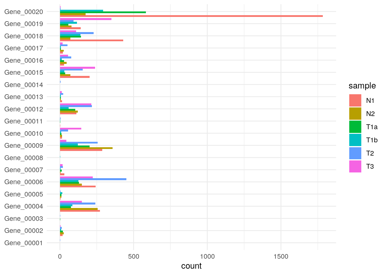
| Version | Author | Date |
|---|---|---|
| 3e572d6 | Dave Tang | 2023-07-26 |
Converting long data back to wide data can be done using
pivot_wider.
tidyr::pivot_wider(
  data = gene_exp_long,
  id_cols = gene,
  names_from = sample,
  values_from = count
)
# A tibble: 18,760 × 7
gene T1a T1b T2 T3 N1 N2
<chr> <int> <int> <int> <int> <int> <int>
1 Gene_00001 0 0 2 0 0 1
2 Gene_00002 20 8 12 5 19 26
3 Gene_00003 3 0 2 0 0 0
4 Gene_00004 75 84 241 149 271 257
5 Gene_00005 10 16 4 0 4 10
6 Gene_00006 129 126 451 223 243 149
7 Gene_00007 13 4 21 19 31 4
8 Gene_00008 0 3 0 0 0 0
9 Gene_00009 202 122 256 43 287 357
10 Gene_00010 10 8 56 145 14 15
# ℹ 18,750 more rowsNow, how do we do this using base R?
Reshape
If you look online for how to mimic the pivot_longer and
pivot_wider functions in base R, you will be introduced to
the reshape() function. The documentation for
reshape() describes the function as:
This function reshapes a data frame between “wide” format (with repeated measurements in separate columns of the same row) and “long” format (with the repeated measurements in separate rows).
The documentation also shows how reshape() is typically
used:
- Typical usage for converting from long to wide format:
# reshape(data, direction = "wide",
#         idvar = "___", timevar = "___", # mandatory
#         v.names = c(___),    # time-varying variables
# varying = list(___)) # auto-generated if missing- Typical usage for converting from wide to long format:
# reshape(data, direction = "long",
#         varying = c(___), # vector
#         sep)              # to help guess 'v.names' and 'times'
Here we convert the wide gene expression data to long format using
reshape.
reshape(
  data = gene_exp,
  direction = "long",
  varying = colnames(gene_exp)[-1],
  v.names = "count",
  times = colnames(gene_exp)[-1],
  timevar = "sample"
) -> out

# order by gene like pivot_longer
out <- out[order(out$gene), ]

# remove row names
row.names(out) <- NULL

# remove id column
out$id <- NULL

head(out)
gene sample count
1 Gene_00001 T1a 0
2 Gene_00001 T1b 0
3 Gene_00001 T2 2
4 Gene_00001 T3 0
5 Gene_00001 N1 0
6 Gene_00001 N2 1table(out$count == gene_exp_long$count)
  TRUE
112560
We achieved the same* result using reshape but with a
bit more typing. (*I simply compared the count values above instead of
using identical or all.equal because
reshape adds attributes to the object that make it
different to the pivot_longer object.)
The arguments for varying and times should
be the column names of the data frame minus the variable to keep
constant. v.names corresponds to values_to and
timevar corresponds to names_to in
pivot_longer.
The reshape() function can also be used to convert long
format back to wide.
reshape(
  data = out,
  direction = "wide",
  idvar = "gene",
  timevar = "sample",
  v.names = "count"
) -> out2

colnames(out2) <- sub("^count\\.", "", colnames(out2))
head(gene_exp)
gene T1a T1b T2 T3 N1 N2
1 Gene_00001 0 0 2 0 0 1
2 Gene_00002 20 8 12 5 19 26
3 Gene_00003 3 0 2 0 0 0
4 Gene_00004 75 84 241 149 271 257
5 Gene_00005 10 16 4 0 4 10
6 Gene_00006 129 126 451 223 243 149head(out2) gene T1a T1b T2 T3 N1 N2
1 Gene_00001 0 0 2 0 0 1
7 Gene_00002 20 8 12 5 19 26
13 Gene_00003 3 0 2 0 0 0
19 Gene_00004 75 84 241 149 271 257
25 Gene_00005 10 16 4 0 4 10
31 Gene_00006 129 126 451 223 243 149It wasn’t obvious to me how I could control the name of the columns
(count is added to the start of the column name) so I
simply added one more line of code to remove the variable name.
Conclusions
R is a statistical language and the design/implementation of functions, their arguments, and documentation reflect this. I’m not a statistician and a lot of the times when I’m reading the documentation for base R functions, it is not immediately obvious to me how I should use it. Personally, Tidyverse packages are more intuitive and easier to use, which is probably the main reason why I prefer it.
However, as I mentioned in the introduction, there are times when I
want an R script to have little to no dependencies. In one of my
scripts, I need to convert data back to wide format and used
pivot_wider. But now I can use the base R function
reshape without having to install the tidyr
package.
Further reading
sessionInfo()R version 4.3.0 (2023-04-21)
Platform: x86_64-pc-linux-gnu (64-bit)
Running under: Ubuntu 22.04.2 LTS
Matrix products: default
BLAS: /usr/lib/x86_64-linux-gnu/openblas-pthread/libblas.so.3
LAPACK: /usr/lib/x86_64-linux-gnu/openblas-pthread/libopenblasp-r0.3.20.so; LAPACK version 3.10.0
locale:
[1] LC_CTYPE=en_US.UTF-8 LC_NUMERIC=C
[3] LC_TIME=en_US.UTF-8 LC_COLLATE=en_US.UTF-8
[5] LC_MONETARY=en_US.UTF-8 LC_MESSAGES=en_US.UTF-8
[7] LC_PAPER=en_US.UTF-8 LC_NAME=C
[9] LC_ADDRESS=C LC_TELEPHONE=C
[11] LC_MEASUREMENT=en_US.UTF-8 LC_IDENTIFICATION=C
time zone: Etc/UTC
tzcode source: system (glibc)
attached base packages:
[1] stats graphics grDevices utils datasets methods base
other attached packages:
[1] ggplot2_3.4.2 tidyr_1.3.0 workflowr_1.7.0
loaded via a namespace (and not attached):
[1] sass_0.4.6 utf8_1.2.3 generics_0.1.3 stringi_1.7.12
[5] digest_0.6.31 magrittr_2.0.3 evaluate_0.21 grid_4.3.0
[9] fastmap_1.1.1 rprojroot_2.0.3 jsonlite_1.8.5 processx_3.8.1
[13] whisker_0.4.1 ps_1.7.5 promises_1.2.0.1 httr_1.4.6
[17] purrr_1.0.1 fansi_1.0.4 scales_1.2.1 jquerylib_0.1.4
[21] cli_3.6.1 rlang_1.1.1 munsell_0.5.0 withr_2.5.0
[25] cachem_1.0.8 yaml_2.3.7 tools_4.3.0 dplyr_1.1.2
[29] colorspace_2.1-0 httpuv_1.6.11 vctrs_0.6.2 R6_2.5.1
[33] lifecycle_1.0.3 git2r_0.32.0 stringr_1.5.0 fs_1.6.2
[37] pkgconfig_2.0.3 callr_3.7.3 pillar_1.9.0 bslib_0.5.0
[41] later_1.3.1 gtable_0.3.3 glue_1.6.2 Rcpp_1.0.10
[45] highr_0.10 xfun_0.39 tibble_3.2.1 tidyselect_1.2.0
[49] rstudioapi_0.14 knitr_1.43 farver_2.1.1 htmltools_0.5.5
[53] rmarkdown_2.22 labeling_0.4.2 compiler_4.3.0 getPass_0.2-2