Finding Markers with Seurat
2025-02-19
Last updated: 2025-02-19
Checks: 7 0
Knit directory: muse/
This reproducible R Markdown analysis was created with workflowr (version 1.7.1). The Checks tab describes the reproducibility checks that were applied when the results were created. The Past versions tab lists the development history.
Great! Since the R Markdown file has been committed to the Git repository, you know the exact version of the code that produced these results.
Great job! The global environment was empty. Objects defined in the global environment can affect the analysis in your R Markdown file in unknown ways. For reproduciblity it’s best to always run the code in an empty environment.
The command set.seed(20200712) was run prior to running
the code in the R Markdown file. Setting a seed ensures that any results
that rely on randomness, e.g. subsampling or permutations, are
reproducible.
Great job! Recording the operating system, R version, and package versions is critical for reproducibility.
Nice! There were no cached chunks for this analysis, so you can be confident that you successfully produced the results during this run.
Great job! Using relative paths to the files within your workflowr project makes it easier to run your code on other machines.
Great! You are using Git for version control. Tracking code development and connecting the code version to the results is critical for reproducibility.
The results in this page were generated with repository version 7ed67d0. See the Past versions tab to see a history of the changes made to the R Markdown and HTML files.
Note that you need to be careful to ensure that all relevant files for
the analysis have been committed to Git prior to generating the results
(you can use wflow_publish or
wflow_git_commit). workflowr only checks the R Markdown
file, but you know if there are other scripts or data files that it
depends on. Below is the status of the Git repository when the results
were generated:
Ignored files:
    Ignored:    .Rproj.user/
    Ignored:    data/1M_neurons_filtered_gene_bc_matrices_h5.h5
    Ignored:    data/293t/
    Ignored:    data/293t_3t3_filtered_gene_bc_matrices.tar.gz
    Ignored:    data/293t_filtered_gene_bc_matrices.tar.gz
    Ignored:    data/5k_Human_Donor1_PBMC_3p_gem-x_5k_Human_Donor1_PBMC_3p_gem-x_count_sample_filtered_feature_bc_matrix.h5
    Ignored:    data/5k_Human_Donor2_PBMC_3p_gem-x_5k_Human_Donor2_PBMC_3p_gem-x_count_sample_filtered_feature_bc_matrix.h5
    Ignored:    data/5k_Human_Donor3_PBMC_3p_gem-x_5k_Human_Donor3_PBMC_3p_gem-x_count_sample_filtered_feature_bc_matrix.h5
    Ignored:    data/5k_Human_Donor4_PBMC_3p_gem-x_5k_Human_Donor4_PBMC_3p_gem-x_count_sample_filtered_feature_bc_matrix.h5
    Ignored:    data/Parent_SC3v3_Human_Glioblastoma_filtered_feature_bc_matrix.tar.gz
    Ignored:    data/brain_counts/
    Ignored:    data/cl.obo
    Ignored:    data/cl.owl
    Ignored:    data/jurkat/
    Ignored:    data/jurkat:293t_50:50_filtered_gene_bc_matrices.tar.gz
    Ignored:    data/jurkat_293t/
    Ignored:    data/jurkat_filtered_gene_bc_matrices.tar.gz
    Ignored:    data/pbmc3k/
    Ignored:    data/pbmc4k_filtered_gene_bc_matrices.tar.gz
    Ignored:    data/refdata-gex-GRCh38-2020-A.tar.gz
    Ignored:    data/seurat_1m_neuron.rds
    Ignored:    data/t_3k_filtered_gene_bc_matrices.tar.gz
    Ignored:    r_packages_4.4.1/
Note that any generated files, e.g. HTML, png, CSS, etc., are not included in this status report because it is ok for generated content to have uncommitted changes.
These are the previous versions of the repository in which changes were
made to the R Markdown (analysis/seurat_markers.Rmd) and
HTML (docs/seurat_markers.html) files. If you’ve configured
a remote Git repository (see ?wflow_git_remote), click on
the hyperlinks in the table below to view the files as they were in that
past version.
| File | Version | Author | Date | Message |
|---|---|---|---|---|
| Rmd | 7ed67d0 | Dave Tang | 2025-02-19 | Features for add module score need to be in a list |
| html | 61c73f8 | Dave Tang | 2025-02-19 | Build site. |
| Rmd | 1349d0c | Dave Tang | 2025-02-19 | CD 8 markers |
| html | 3c2f9fa | Dave Tang | 2025-01-16 | Build site. |
| Rmd | 380f7f8 | Dave Tang | 2025-01-16 | Remove unnecessary output |
| html | e2a1a6b | Dave Tang | 2025-01-16 | Build site. |
| Rmd | cd0f44f | Dave Tang | 2025-01-16 | Module scores |
| html | 72b0d6d | Dave Tang | 2025-01-15 | Build site. |
| Rmd | bcb5c7b | Dave Tang | 2025-01-15 | Manually use {presto} to calculate pvalues |
| html | 8539125 | Dave Tang | 2025-01-15 | Build site. |
| Rmd | 240ee62 | Dave Tang | 2025-01-15 | Compare p-value calculations |
| html | 50fef6c | Dave Tang | 2025-01-15 | Build site. |
| Rmd | cb2011a | Dave Tang | 2025-01-15 | FindMarkers with groups |
| html | 522ba27 | Dave Tang | 2024-12-25 | Build site. |
| Rmd | ecf10e9 | Dave Tang | 2024-12-25 | FindMarkers in parallel |
| html | 612e4f9 | Dave Tang | 2024-12-24 | Build site. |
| Rmd | f0f7a57 | Dave Tang | 2024-12-24 | Finding Markers with Seurat |
Use the Peripheral Blood Mononuclear Cells (PBMCs) 2,700 cells dataset to test finding markers with Seurat.
Install the following packages, if necessary.
install.packages("remotes")
remotes::install_github("immunogenomics/presto")
install.packages("Seurat")
install.packages("bench")
Load Seurat and bench for some
benchmarking.
suppressPackageStartupMessages(library("Seurat"))
suppressPackageStartupMessages(library("bench"))
suppressPackageStartupMessages(library("presto"))
suppressPackageStartupMessages(library("ggplot2"))
Data
To follow the tutorial, you’ll need the 10X data, which can be download from AWS.
mkdir -p data/pbmc3k && cd data/pbmc3k
wget -c https://s3-us-west-2.amazonaws.com/10x.files/samples/cell/pbmc3k/pbmc3k_filtered_gene_bc_matrices.tar.gz
tar -xzf pbmc3k_filtered_gene_bc_matrices.tar.gz
Seurat object
Load 10x data into a matrix using Read10X().
work_dir <- rprojroot::find_rstudio_root_file()
data_dir <- paste0(work_dir, "/data/pbmc3k/filtered_gene_bc_matrices/hg19/")
stopifnot(dir.exists(data_dir))
pbmc.data <- Read10X(
  data.dir = data_dir
)
Create the Seurat object using CreateSeuratObject; see
?SeuratObject for more information on the class.
seurat_obj <- CreateSeuratObject(
  counts = pbmc.data,
  min.cells = 3,
  min.features = 200,
  project = "pbmc3k"
)
Warning: Feature names cannot have underscores ('_'), replacing with dashes
('-')class(seurat_obj)[1] "Seurat"
attr(,"package")
[1] "SeuratObject"Seurat workflow
Run the workflow as separate steps; they can be piped together but sometimes errors occur, so it is useful to split up the steps.
debug_flag <- FALSE
seurat_obj <- NormalizeData(seurat_obj, normalization.method = "LogNormalize", scale.factor = 1e4, verbose = debug_flag)
seurat_obj <- FindVariableFeatures(seurat_obj, selection.method = 'vst', nfeatures = 2000, verbose = debug_flag)
seurat_obj <- ScaleData(seurat_obj, verbose = debug_flag)
seurat_obj <- RunPCA(seurat_obj, verbose = debug_flag)
seurat_obj <- RunUMAP(seurat_obj, dims = 1:30, verbose = debug_flag)
Warning: The default method for RunUMAP has changed from calling Python UMAP via reticulate to the R-native UWOT using the cosine metric
To use Python UMAP via reticulate, set umap.method to 'umap-learn' and metric to 'correlation'
This message will be shown once per sessionseurat_obj <- FindNeighbors(seurat_obj, dims = 1:30, verbose = debug_flag)
seurat_obj <- FindClusters(seurat_obj, resolution = 0.5, verbose = debug_flag)
seurat_objAn object of class Seurat
13714 features across 2700 samples within 1 assay
Active assay: RNA (13714 features, 2000 variable features)
3 layers present: counts, data, scale.data
2 dimensional reductions calculated: pca, umapKnown markers
UMAP.
DimPlot(seurat_obj, label = TRUE)
| Version | Author | Date |
|---|---|---|
| 61c73f8 | Dave Tang | 2025-02-19 |
Known markers.
known_markers <- tibble::tribble(
  ~Label, ~`Expanded Label`, ~`OBO Ontology ID`, ~Markers,
  "Mono", "Monocyte", "CL:0000576", "CTSS, FCN1, NEAT1, LYZ, PSAP, S100A9, AIF1, MNDA, SERPINA1, TYROBP",
  "CD4 T", "CD4+ T cell", "CL:0000624", "IL7R, MAL, LTB, CD4, LDHB, TPT1, TRAC, TMSB10, CD3D, CD3G",
  "CD8 T", "CD8+ T cell", "CL:0000625", "CD8B, CD8A, CD3D, TMSB10, HCST, CD3G, LINC02446, CTSW, CD3E, TRAC",
  "NK", "natural killer cell", "CL:0000623", "NKG7, KLRD1, TYROBP, GNLY, FCER1G, PRF1, CD247, KLRF1, CST7, GZMB",
  "B", "B cell", "CL:0000785", "CD79A, RALGPS2, CD79B, MS4A1, BANK1, CD74, TNFRSF13C, HLA-DQA1, IGHM, MEF2C",
  "other T", "other T cell", "CL:0002419", "CD3D, TRDC, GZMK, KLRB1, NKG7, TRGC2, CST7, LYAR, KLRG1, GZMA",
  "DC", "dendritic cell", "CL:0000451", "CD74, HLA-DPA1, HLA-DPB1, HLA-DQA1, CCDC88A, HLA-DRA, HLA-DMA, CST3, HLA-DQB1, HLA-DRB1"
)

known_markers
# A tibble: 7 × 4
Label `Expanded Label` `OBO Ontology ID` Markers
<chr> <chr> <chr> <chr>
1 Mono Monocyte CL:0000576 CTSS, FCN1, NEAT1, LYZ, PSAP, S…
2 CD4 T CD4+ T cell CL:0000624 IL7R, MAL, LTB, CD4, LDHB, TPT1…
3 CD8 T CD8+ T cell CL:0000625 CD8B, CD8A, CD3D, TMSB10, HCST,…
4 NK natural killer cell CL:0000623 NKG7, KLRD1, TYROBP, GNLY, FCER…
5 B B cell CL:0000785 CD79A, RALGPS2, CD79B, MS4A1, B…
6 other T other T cell CL:0002419 CD3D, TRDC, GZMK, KLRB1, NKG7, …
7 DC dendritic cell CL:0000451 CD74, HLA-DPA1, HLA-DPB1, HLA-D…Plot CD8 markers.
known_markers |>
  dplyr::filter(Label == "CD8 T") |>
  dplyr::pull(Markers) |>
  stringr::str_split(pattern = ", ") |>
  unlist() -> cd8_markers

Seurat::FeaturePlot(seurat_obj, features = cd8_markers)
Warning: The following requested variables were not found: LINC02446, TRAC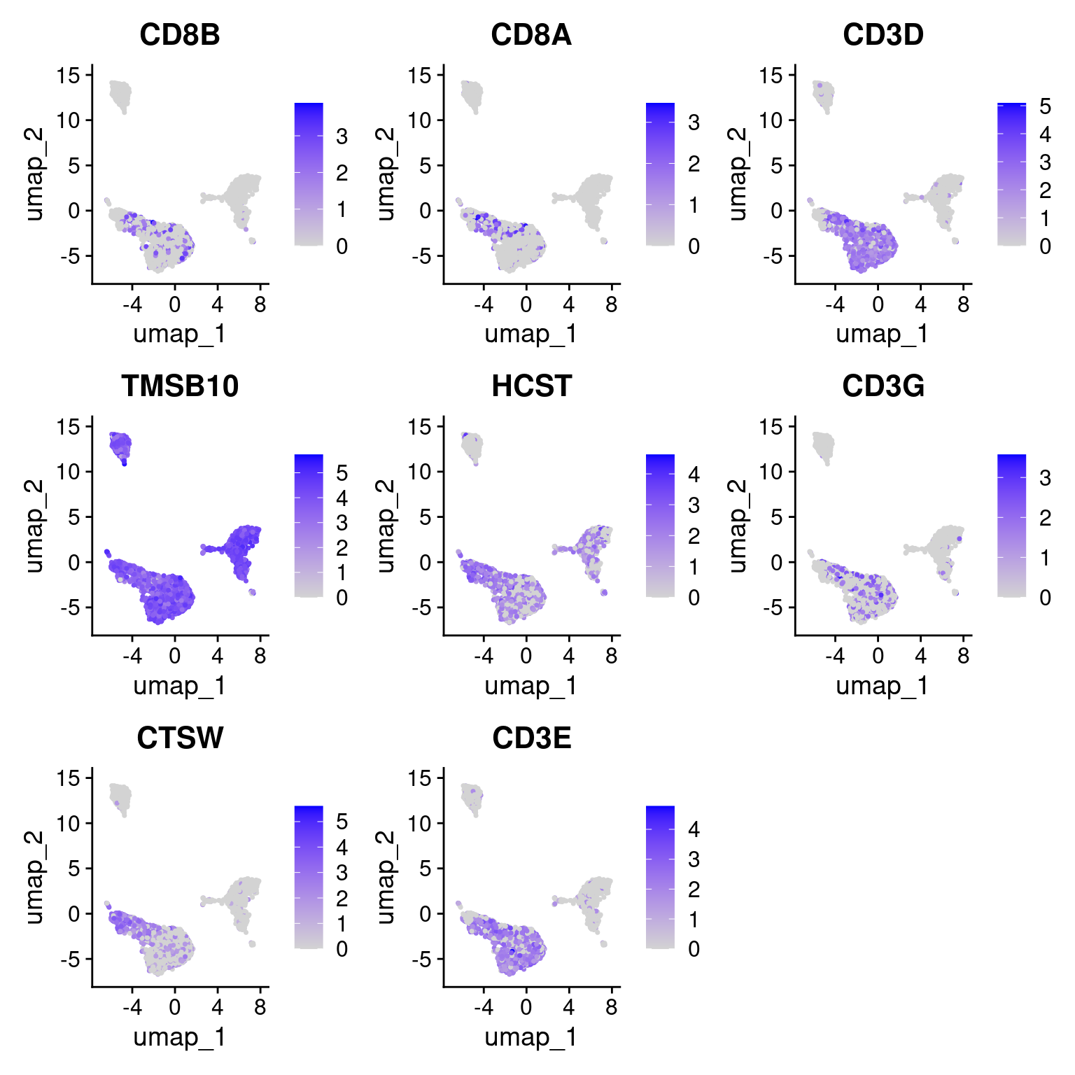
| Version | Author | Date |
|---|---|---|
| 61c73f8 | Dave Tang | 2025-02-19 |
Find all markers
FindAllMarkers() will find markers (differentially
expressed genes) for each of the identity classes in a dataset.
levels(Idents(seurat_obj))[1] "0" "1" "2" "3" "4" "5" "6" "7"Find all markers.
all_markers <- FindAllMarkers(seurat_obj, verbose = debug_flag)
dim(all_markers)
[1] 17899 7Find markers
FindMarkers() finds markers (differentially expressed
genes) for identity classes. Things to note:
- Default is to use the
dataslot/layer; this contains normalised values (after runningNormalizeData()) ident.1- Identity class to define markers for; pass an object of classphyloorclustertreeto find markers for a node in a cluster tree; passingclustertreerequiresBuildClusterTree()to have been runident.2- A second identity class for comparison; if NULL, use all other cells for comparison; if an object of classphyloorclustertreeis passed toident.1, must pass a node to find markers forgroup.by- Regroup cells into a different identity class prior to performing differential expressionsubset.ident- Subset a particular identity class prior to regrouping. Only relevant if group.by is set
pbmc_small
pbmc_small dataset.
data(pbmc_small)
pbmc_small
An object of class Seurat
230 features across 80 samples within 1 assay
Active assay: RNA (230 features, 20 variable features)
3 layers present: counts, data, scale.data
2 dimensional reductions calculated: pca, tsnepbmc_small metadata.
table(
  pbmc_small@meta.data$RNA_snn_res.1,
  pbmc_small@meta.data$groups
)
    g1 g2
  0 20 16
  1 14 11
  2 10  9
Take all cells in cluster 2, and find markers that separate cells in the ‘g1’ group (metadata variable ‘group’).
pbmc_small_markers <- FindMarkers(pbmc_small, ident.1 = "g1", group.by = 'groups', subset.ident = "2")
head(pbmc_small_markers)
p_val avg_log2FC pct.1 pct.2 p_val_adj
GSTP1 0.01601528 2.603521 0.7 0.111 1
LINC00936 0.02048683 7.182496 0.5 0.000 1
TPM4 0.02048683 7.488007 0.5 0.000 1
LGALS2 0.04515259 7.403075 0.4 0.000 1
IFI30 0.04515259 7.794332 0.4 0.000 1
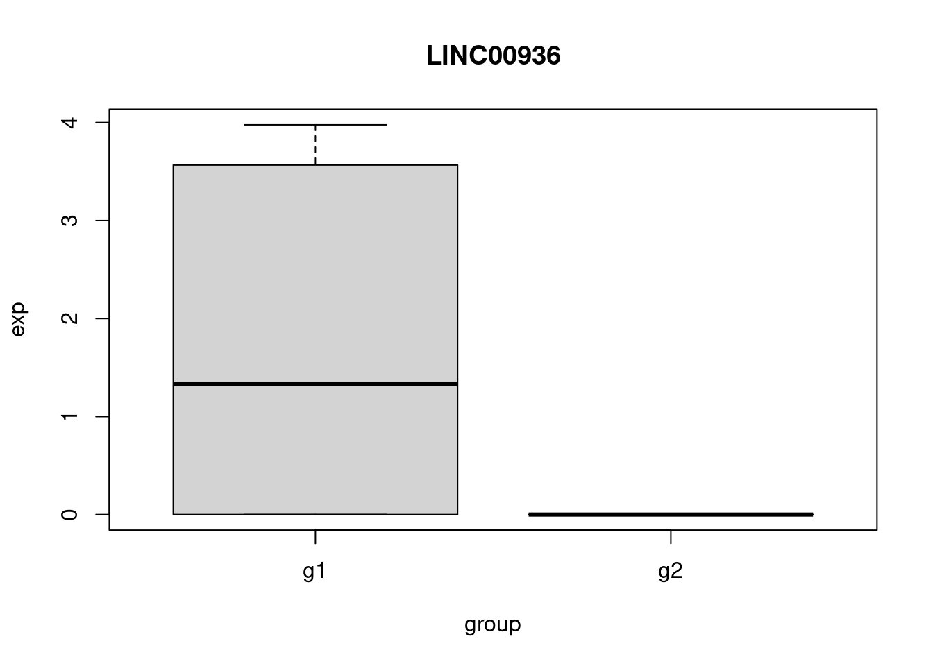
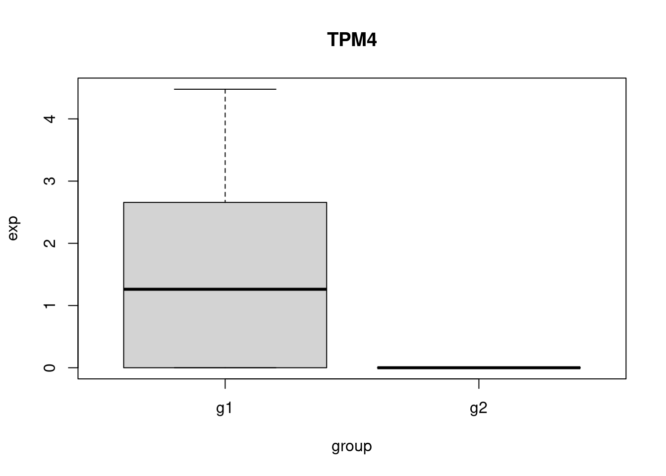
RHOC 0.04515259 7.016294 0.4 0.000 1Perform some sanity checks.
get_exp <- function(gene){
  gene_exp <- pbmc_small[['RNA']]['data'][gene, ]

  pbmc_small@meta.data |>
    dplyr::filter(RNA_snn_res.1 == 2, groups == 'g1') |>
    row.names() -> g1_c2

  pbmc_small@meta.data |>
    dplyr::filter(RNA_snn_res.1 == 2, groups == 'g2') |>
    row.names() -> g2_c2

  g1 <- gene_exp[g1_c2]
  g2 <- gene_exp[g2_c2]
  rbind(
    data.frame(exp = g1, group = "g1"),
    data.frame(exp = g2, group = "g2")
  )
}

plot_gene <- function(gene){
  my_df <- get_exp(gene)

  boxplot(
    exp~group,
    data = my_df,
    main = gene
  )
}

head(pbmc_small_markers, 3) |>
  row.names() -> genes_to_check

sapply(genes_to_check, plot_gene) -> dev_null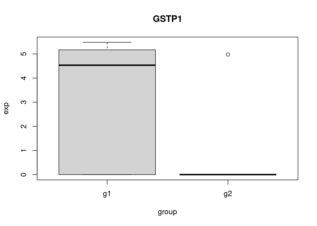
| Version | Author | Date |
|---|---|---|
| 50fef6c | Dave Tang | 2025-01-15 |
| Version | Author | Date |
|---|---|---|
| 50fef6c | Dave Tang | 2025-01-15 |
| Version | Author | Date |
|---|---|---|
| 50fef6c | Dave Tang | 2025-01-15 |
Perform Wilcoxon Rank Sum and Signed Rank Tests using
wilcox.test and compare results.
purrr::map_dbl(row.names(pbmc_small_markers), \(x){
  wilcox.test(exp~group, data = get_exp(x))$p.value
}) |>
  suppressWarnings() -> manual_p_values

plot(pbmc_small_markers$p_val, manual_p_values, pch = 16)
abline(a = 0, b = 1, lty = 2, col = 2)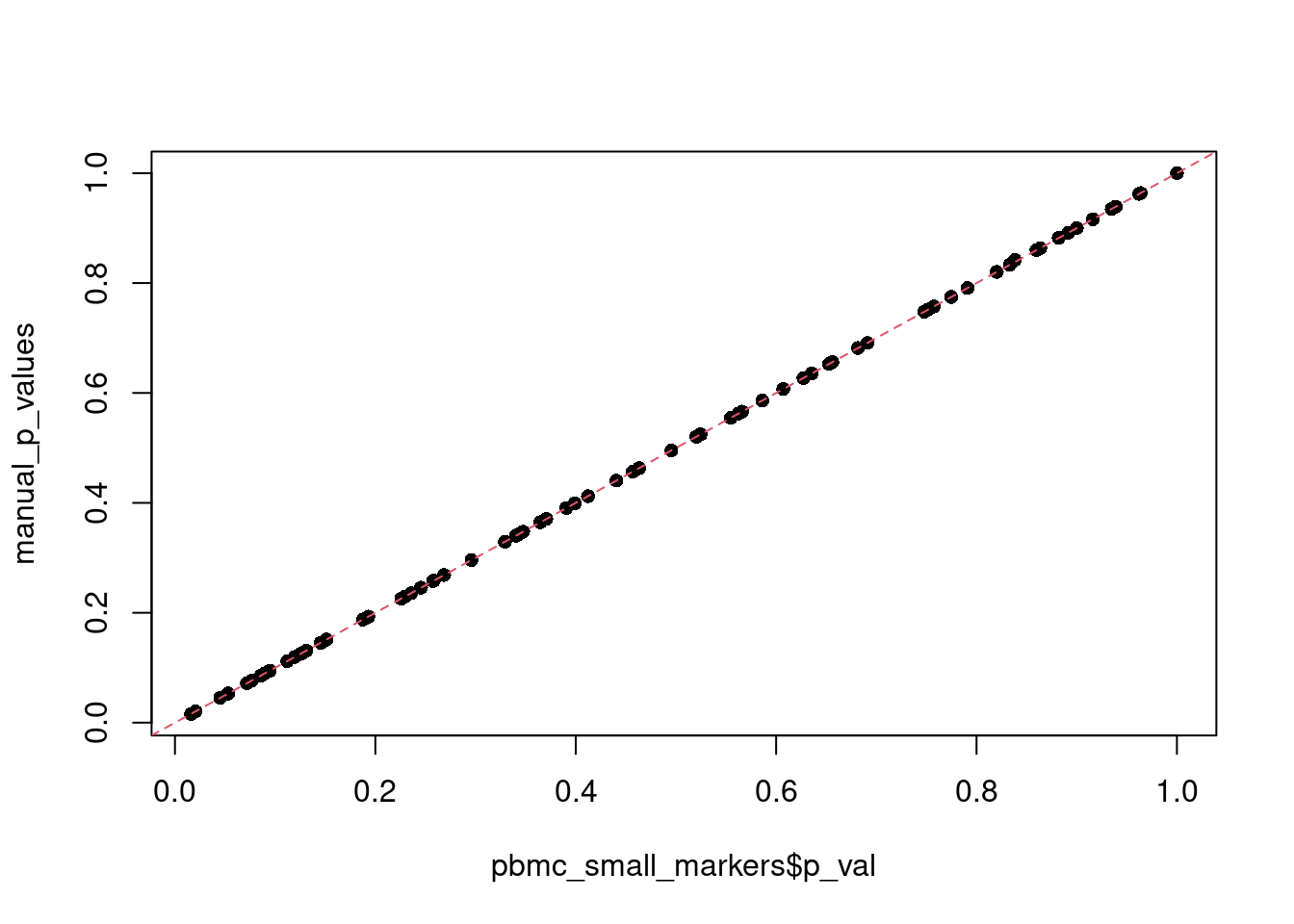
Fast Wilcoxon rank sum test and auROC using
presto::wilcoxauc().
run_presto_wilcox <- function(gene){
  wanted <- pbmc_small@meta.data$RNA_snn_res.1 == "2"
  seurat_obj <- pbmc_small[, wanted]

  seurat_obj[['RNA']]$data |>
    as.matrix() -> data_mat

  my_exp <- data_mat[gene, ]
  my_mat <- matrix(my_exp, nrow = 1)
  colnames(my_mat) <- names(my_exp)
  rownames(my_mat) <- gene
  y <- factor(seurat_obj@meta.data$groups)
  res <- presto::wilcoxauc(my_mat, y)
  res <- res[1:(nrow(x = res)/2),]
  res$pval
}

purrr::map_dbl(row.names(pbmc_small_markers), run_presto_wilcox) -> presto_p_values

plot(pbmc_small_markers$p_val, presto_p_values, pch = 16)
abline(a = 0, b = 1, lty = 2, col = 2)
p-value adjustment is performed using bonferroni correction based on the total number of genes in the dataset. Other correction methods are not recommended, as Seurat pre-filters genes using the arguments above, reducing the number of tests performed. Lastly, as Aaron Lun has pointed out, p-values should be interpreted cautiously, as the genes used for clustering are the same genes tested for differential expression.
all(p.adjust(manual_p_values, method = "bonferroni") == pbmc_small_markers$p_val_adj)[1] TRUEpbmc3k
Find markers for cluster 0 in pbmc3k.
cluster_0_markers <- FindMarkers(seurat_obj, ident.1 = "0")
dim(cluster_0_markers)
[1] 8434 5Cluster 0 markers from FindAllMarkers().
all_markers |>
  dplyr::filter(cluster == 0) |>
  dim()
[1] 3139 7The start of the results are the same.
head(cluster_0_markers) p_val avg_log2FC pct.1 pct.2 p_val_adj
LDHB 1.547138e-240 1.9351689 0.922 0.473 2.121746e-236
RPS12 3.595829e-228 0.8665851 1.000 0.987 4.931320e-224
CD74 2.127919e-225 -3.1636831 0.735 0.925 2.918227e-221
HLA-DRB1 3.113535e-225 -4.3722870 0.129 0.715 4.269901e-221
CYBA 2.054958e-213 -1.8108145 0.730 0.933 2.818169e-209
HLA-DRA 7.109002e-213 -4.6393725 0.291 0.765 9.749286e-209all_markers |>
dplyr::filter(cluster == 0) |>
dplyr::select(-cluster, -gene) |>
head() p_val avg_log2FC pct.1 pct.2 p_val_adj
LDHB 1.547138e-240 1.9351689 0.922 0.473 2.121746e-236
RPS12 3.595829e-228 0.8665851 1.000 0.987 4.931320e-224
CD74 2.127919e-225 -3.1636831 0.735 0.925 2.918227e-221
HLA-DRB1 3.113535e-225 -4.3722870 0.129 0.715 4.269901e-221
CYBA 2.054958e-213 -1.8108145 0.730 0.933 2.818169e-209
HLA-DRA 7.109002e-213 -4.6393725 0.291 0.765 9.749286e-209The tail of the results are the same too, except that in
FindAllMarkers() results have been trimmed.
cluster_0_markers[3134:3139, ] p_val avg_log2FC pct.1 pct.2 p_val_adj
SCML1 0.009913768 1.2125839 0.028 0.014 1
CGGBP1 0.009914211 0.3048076 0.152 0.117 1
CCT3 0.009950407 0.2610577 0.231 0.190 1
ZNF32 0.009955859 0.1339321 0.108 0.079 1
RNF214 0.009977100 0.8208791 0.043 0.025 1
P2RX7 0.009979523 -1.7709166 0.003 0.013 1all_markers |>
dplyr::filter(cluster == 0) |>
dplyr::select(-cluster, -gene) |>
tail() p_val avg_log2FC pct.1 pct.2 p_val_adj
SCML1 0.009913768 1.2125839 0.028 0.014 1
CGGBP1 0.009914211 0.3048076 0.152 0.117 1
CCT3 0.009950407 0.2610577 0.231 0.190 1
ZNF32 0.009955859 0.1339321 0.108 0.079 1
RNF214 0.009977100 0.8208791 0.043 0.025 1
P2RX7 0.009979523 -1.7709166 0.003 0.013 1Trimming seems to be from p_val < 0.01
cluster_0_markers[3139:3142, ] p_val avg_log2FC pct.1 pct.2 p_val_adj
P2RX7 0.009979523 -1.7709166 0.003 0.013 1
CBFB 0.010029322 0.6492086 0.068 0.046 1
ATF6B 0.010045052 -0.4047457 0.130 0.165 1
PCNT 0.010051913 -1.8088730 0.003 0.013 1Find markers in parallel to speed up FindAllMarkers().
Use imap() to get the name of each list (.y);
.x is each element of the list.
library(future)
library(future.apply)

clusters <- levels(Idents(seurat_obj))
plan(multisession, workers = 4)
markers <- future_lapply(
  clusters,
  function(x){
    FindMarkers(seurat_obj, ident.1 = x)
  },
  future.seed = TRUE
)

names(markers) <- clusters

purrr::map(
  markers,
  \(x) tibble::rownames_to_column(.data = x, var = "gene") |> tibble::remove_rownames()
) |>
  purrr::imap(~ dplyr::mutate(.x, cluster = .y)) |>
  purrr::list_rbind() |>
  dplyr::filter(p_val < 0.01) |>
  dplyr::mutate(cluster = factor(cluster, levels = clusters)) |>
  dplyr::select(p_val, avg_log2FC, pct.1, pct.2, p_val_adj, cluster, gene) -> all_markers_parallel

all.equal(
  all_markers_parallel,
  tibble::remove_rownames(all_markers)
)
[1] TRUECalculate module scores
The function AddModuleScore():
Calculate the average expression levels of each program (cluster) on single cell level, subtracted by the aggregated expression of control feature sets. All analyzed features are binned based on averaged expression, and the control features are randomly selected from each bin.
Arguments:
object- Seurat objectfeatures- A list of vectors of features for expression programs; each entry should be a vector of feature namespool- List of features to check expression levels against, defaults to rownames(x = object)nbin- Number of bins of aggregate expression levels for all analyzed featuresctrl- Number of control features selected from the same bin per analyzed featurek- Use feature clusters returned from DoKMeansassay- Name of assay to usename- Name for the expression programs; will append a number to the end for each entry in features (eg. if features has three programs, the results will be stored as name1, name2, name3, respectively)seed- Set a random seed. If NULL, seed is not set.search- Search for symbol synonyms for features in features that don’t match features in object? Searches the HGNC’s gene names database; see UpdateSymbolList for more detailsslot- Slot to calculate score values off of. Defaults to data slot (i.e log-normalized counts)
pbmc_small_markers |>
  head(10) |>
  row.names() -> my_features
feature_list <- list(my_features)

AddModuleScore(
  object = pbmc_small,
  features = feature_list,
  ctrl = 5,
  name = 'cluster_2_markers'
) -> pbmc_small
Plot module scores; feature_list contains genes that are
markers for g1 within cluster 2. The boxplot confirms the
results by showing higher module scores in cluster 2 of g1.
ggplot(pbmc_small@meta.data, aes(RNA_snn_res.1, cluster_2_markers1)) +
  geom_boxplot() +
  theme_minimal() +
  facet_grid(~groups)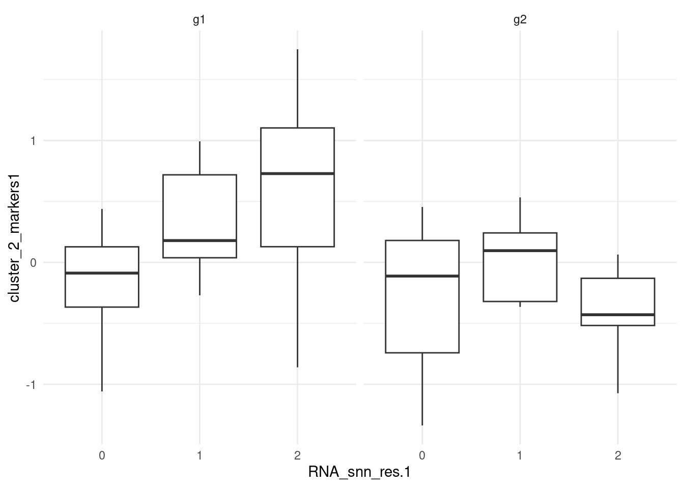
| Version | Author | Date |
|---|---|---|
| e2a1a6b | Dave Tang | 2025-01-16 |
Visualise module scores on the UMAP.
pbmc_small <- RunUMAP(object = pbmc_small, dims = 1:19, verbose = FALSE)

cbind(
  pbmc_small@meta.data,
  pbmc_small@reductions$umap@cell.embeddings[, 1:2]
) |>
  ggplot(aes(umap_1, umap_2, colour = cluster_2_markers1, shape = RNA_snn_res.1)) +
  geom_point() +
  theme_minimal() +
  facet_grid(~groups)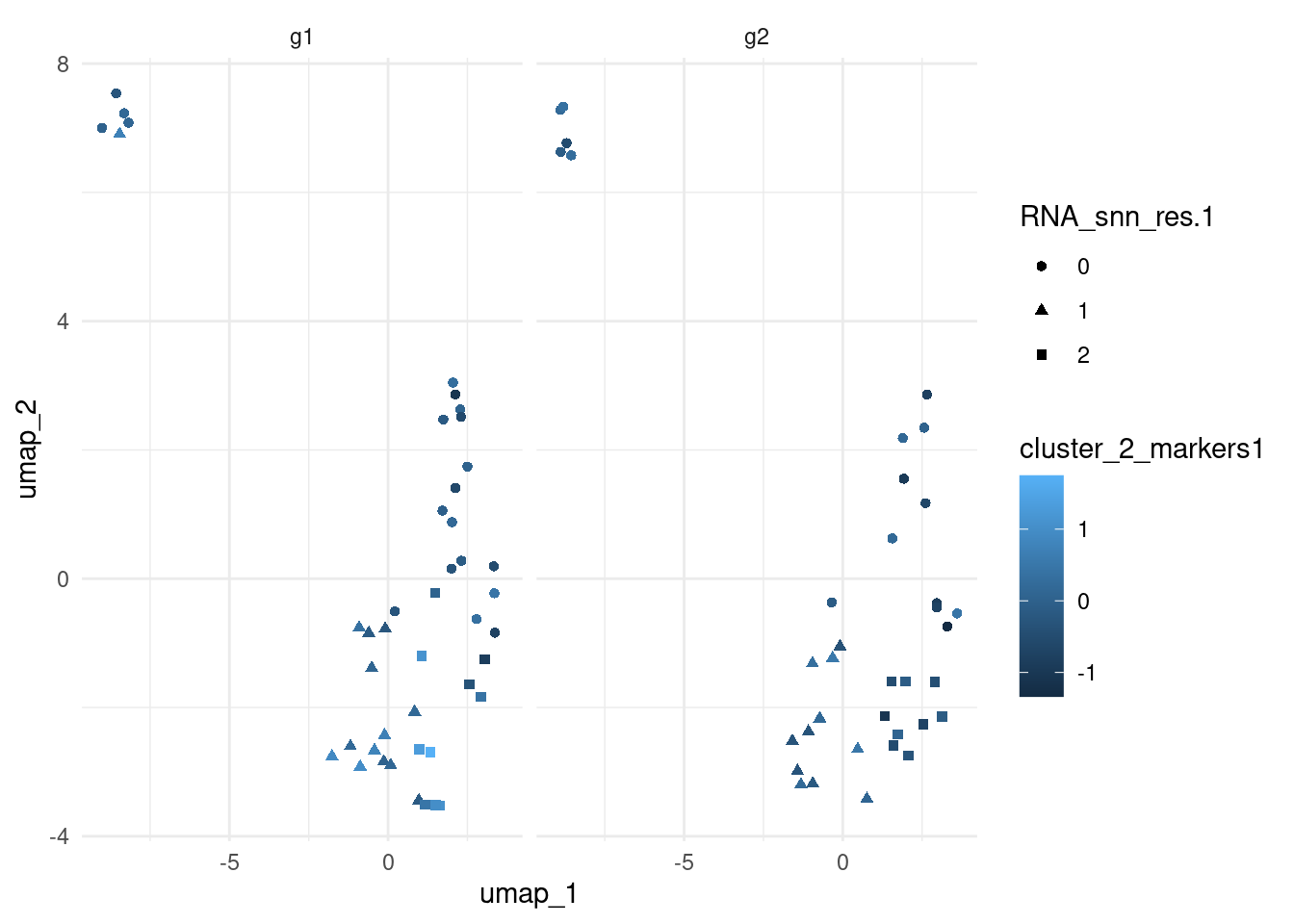
| Version | Author | Date |
|---|---|---|
| e2a1a6b | Dave Tang | 2025-01-16 |
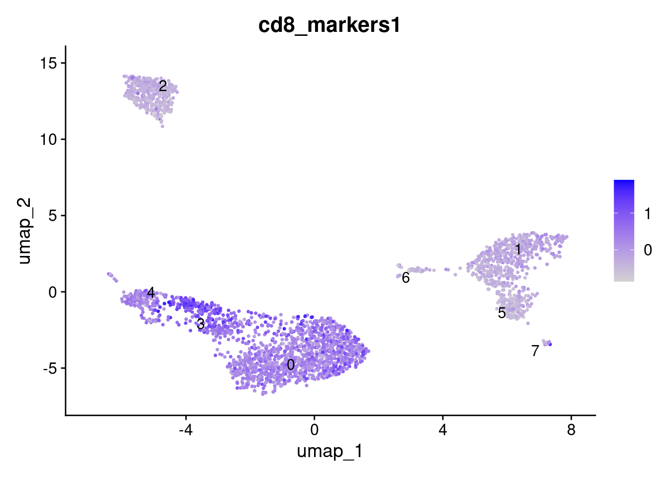
CD 8
Add module score for CD 8 markers.
cd8_markers_found <- cd8_markers[cd8_markers %in% row.names(seurat_obj@assays$RNA$data)]

AddModuleScore(
  object = seurat_obj,
  features = list(cd8_markers_found),
  name = 'cd8_markers'
) -> seurat_obj

FeaturePlot(
  seurat_obj,
  features = "cd8_markers1", label = TRUE, repel = TRUE
)
| Version | Author | Date |
|---|---|---|
| 61c73f8 | Dave Tang | 2025-02-19 |
sessionInfo()R version 4.4.1 (2024-06-14)
Platform: x86_64-pc-linux-gnu
Running under: Ubuntu 22.04.5 LTS
Matrix products: default
BLAS: /usr/lib/x86_64-linux-gnu/openblas-pthread/libblas.so.3
LAPACK: /usr/lib/x86_64-linux-gnu/openblas-pthread/libopenblasp-r0.3.20.so; LAPACK version 3.10.0
locale:
[1] LC_CTYPE=en_US.UTF-8 LC_NUMERIC=C
[3] LC_TIME=en_US.UTF-8 LC_COLLATE=en_US.UTF-8
[5] LC_MONETARY=en_US.UTF-8 LC_MESSAGES=en_US.UTF-8
[7] LC_PAPER=en_US.UTF-8 LC_NAME=C
[9] LC_ADDRESS=C LC_TELEPHONE=C
[11] LC_MEASUREMENT=en_US.UTF-8 LC_IDENTIFICATION=C
time zone: Etc/UTC
tzcode source: system (glibc)
attached base packages:
[1] stats graphics grDevices utils datasets methods base
other attached packages:
[1] future.apply_1.11.3 future_1.34.0 ggplot2_3.5.1
[4] presto_1.0.0 data.table_1.16.2 Rcpp_1.0.13
[7] bench_1.1.3 Seurat_5.1.0 SeuratObject_5.0.2
[10] sp_2.1-4 workflowr_1.7.1
loaded via a namespace (and not attached):
[1] RColorBrewer_1.1-3 rstudioapi_0.17.1 jsonlite_1.8.9
[4] magrittr_2.0.3 spatstat.utils_3.1-0 farver_2.1.2
[7] rmarkdown_2.28 fs_1.6.4 vctrs_0.6.5
[10] ROCR_1.0-11 spatstat.explore_3.3-3 htmltools_0.5.8.1
[13] sass_0.4.9 sctransform_0.4.1 parallelly_1.38.0
[16] KernSmooth_2.23-24 bslib_0.8.0 htmlwidgets_1.6.4
[19] ica_1.0-3 plyr_1.8.9 plotly_4.10.4
[22] zoo_1.8-12 cachem_1.1.0 whisker_0.4.1
[25] igraph_2.1.1 mime_0.12 lifecycle_1.0.4
[28] pkgconfig_2.0.3 Matrix_1.7-0 R6_2.5.1
[31] fastmap_1.2.0 fitdistrplus_1.2-1 shiny_1.9.1
[34] digest_0.6.37 colorspace_2.1-1 patchwork_1.3.0
[37] ps_1.8.1 rprojroot_2.0.4 tensor_1.5
[40] RSpectra_0.16-2 irlba_2.3.5.1 labeling_0.4.3
[43] progressr_0.15.0 fansi_1.0.6 spatstat.sparse_3.1-0
[46] httr_1.4.7 polyclip_1.10-7 abind_1.4-8
[49] compiler_4.4.1 withr_3.0.2 fastDummies_1.7.4
[52] highr_0.11 R.utils_2.12.3 MASS_7.3-60.2
[55] tools_4.4.1 lmtest_0.9-40 httpuv_1.6.15
[58] goftest_1.2-3 R.oo_1.26.0 glue_1.8.0
[61] callr_3.7.6 nlme_3.1-164 promises_1.3.0
[64] grid_4.4.1 Rtsne_0.17 getPass_0.2-4
[67] cluster_2.1.6 reshape2_1.4.4 generics_0.1.3
[70] gtable_0.3.6 spatstat.data_3.1-2 R.methodsS3_1.8.2
[73] tidyr_1.3.1 utf8_1.2.4 spatstat.geom_3.3-3
[76] RcppAnnoy_0.0.22 ggrepel_0.9.6 RANN_2.6.2
[79] pillar_1.9.0 stringr_1.5.1 limma_3.62.2
[82] spam_2.11-0 RcppHNSW_0.6.0 later_1.3.2
[85] splines_4.4.1 dplyr_1.1.4 lattice_0.22-6
[88] survival_3.6-4 deldir_2.0-4 tidyselect_1.2.1
[91] miniUI_0.1.1.1 pbapply_1.7-2 knitr_1.48
[94] git2r_0.35.0 gridExtra_2.3 scattermore_1.2
[97] xfun_0.48 statmod_1.5.0 matrixStats_1.4.1
[100] stringi_1.8.4 lazyeval_0.2.2 yaml_2.3.10
[103] evaluate_1.0.1 codetools_0.2-20 tibble_3.2.1
[106] cli_3.6.3 uwot_0.2.2 xtable_1.8-4
[109] reticulate_1.39.0 munsell_0.5.1 processx_3.8.4
[112] jquerylib_0.1.4 globals_0.16.3 spatstat.random_3.3-2
[115] png_0.1-8 spatstat.univar_3.0-1 parallel_4.4.1
[118] dotCall64_1.2 listenv_0.9.1 viridisLite_0.4.2
[121] scales_1.3.0 ggridges_0.5.6 leiden_0.4.3.1
[124] purrr_1.0.2 rlang_1.1.4 cowplot_1.1.3