Survival analysis using the survival and survminer R packages
2023-12-20
Last updated: 2023-12-20
Checks: 7 0
Knit directory: muse/
This reproducible R Markdown analysis was created with workflowr (version 1.7.1). The Checks tab describes the reproducibility checks that were applied when the results were created. The Past versions tab lists the development history.
Great! Since the R Markdown file has been committed to the Git repository, you know the exact version of the code that produced these results.
Great job! The global environment was empty. Objects defined in the global environment can affect the analysis in your R Markdown file in unknown ways. For reproduciblity it’s best to always run the code in an empty environment.
The command set.seed(20200712) was run prior to running
the code in the R Markdown file. Setting a seed ensures that any results
that rely on randomness, e.g. subsampling or permutations, are
reproducible.
Great job! Recording the operating system, R version, and package versions is critical for reproducibility.
Nice! There were no cached chunks for this analysis, so you can be confident that you successfully produced the results during this run.
Great job! Using relative paths to the files within your workflowr project makes it easier to run your code on other machines.
Great! You are using Git for version control. Tracking code development and connecting the code version to the results is critical for reproducibility.
The results in this page were generated with repository version 935f552. See the Past versions tab to see a history of the changes made to the R Markdown and HTML files.
Note that you need to be careful to ensure that all relevant files for
the analysis have been committed to Git prior to generating the results
(you can use wflow_publish or
wflow_git_commit). workflowr only checks the R Markdown
file, but you know if there are other scripts or data files that it
depends on. Below is the status of the Git repository when the results
were generated:
Ignored files:
    Ignored:    .Rproj.user/
    Ignored:    r_packages_4.3.2/
Note that any generated files, e.g. HTML, png, CSS, etc., are not included in this status report because it is ok for generated content to have uncommitted changes.
These are the previous versions of the repository in which changes were
made to the R Markdown (analysis/survival.Rmd) and HTML
(docs/survival.html) files. If you’ve configured a remote
Git repository (see ?wflow_git_remote), click on the
hyperlinks in the table below to view the files as they were in that
past version.
| File | Version | Author | Date | Message |
|---|---|---|---|---|
| Rmd | 935f552 | Dave Tang | 2023-12-20 | Add control data |
| html | 3540955 | Dave Tang | 2023-11-09 | Build site. |
| Rmd | 4cfa454 | Dave Tang | 2023-11-09 | Switch status |
| html | 1d0acd6 | Dave Tang | 2023-11-09 | Build site. |
| Rmd | 078c04a | Dave Tang | 2023-11-09 | Use factors for covariates |
| html | 24d29bb | Dave Tang | 2023-11-09 | Build site. |
| Rmd | b4509a9 | Dave Tang | 2023-11-09 | Include additional covariates |
| html | 797564f | Dave Tang | 2023-11-09 | Build site. |
| Rmd | 37e1a56 | Dave Tang | 2023-11-09 | Cox proportional-hazards model |
| html | b1d68db | Dave Tang | 2023-11-09 | Build site. |
| Rmd | 16f2e4c | Dave Tang | 2023-11-09 | Survival analysis |
Introduction
Survival analysis corresponds to a set of statistical approaches used to investigate the time it takes for an event of interest to occur. It is used in:
- Cancer studies for patient’s survival time analysis
- Sociology for event-history analysis
- Engineering for failure-time analysis
In cancer studies, typical research questions include:
- What is the impact of certain clinical characteristics on patient’s survival?
- What is the probability that an individual survives 3 years?
- Are there differences in survival between groups of patients?
Most survival analyses in cancer studies use the following methods:
- Kaplan-Meier plots to visualise survival curves
- Log-rank test to compare the survival curves of two or more groups
- Cox proportional hazards regression to describe the effect of variables on survival
Basic concepts
Survival time and type of events in cancer studies
There are different types of events in cancer studies, including:
- Relapse
- Progression
- Death
The time from “response to treatment” (complete remission) to the occurrence of the event of interest is commonly called survival time (or time to event).
The two most important measures in cancer studies include:
- The time to death
- The relapse-free survival time, which corresponds to the time between response to treatment and recurrence of the disease. It is also known as disease-free survival time and event-free survival time.
Censoring
Survival analysis focuses on the expected duration of time until occurrence of an event of interest (relapse or death). However, the event may not be observed for some individuals within the study time period, producing the so-called censored observations.
Censoring may arise in the following ways:
- A patient has not (yet) experienced the event of interest, such as relapse or death, within the study time period;
- A patient is lost to follow-up during the study period;
- A patient experiences a different event that makes further follow-up impossible.
Survival and hazard functions
Two related probabilities are used to describe survival data:
- The survival probability
- The hazard probability
The survival probability, also known as the survivor function \(S(t)\), is the probability that an individual survives from the time origin (e.g. diagnosis of cancer) to a specified future time \(t\).
The hazard, denoted by \(h(t)\), is the probability that an individual who is under observation at a time \(t\) has an event at that time.
The survivor function focuses on not having an event and the hazard function focuses on the event occurring.
Kaplan-Meier survival estimate
The Kaplan-Meier (KM) method is a non-parametric method used to estimate the survival probability from observed survival times (Kaplan and Meier, 1958).
The survival probability at time \(t_i\), \(S(t_i)\) is calculated as follows:
\[ S(t_i) = S(t_{i-1})(1 - \frac{d_i}{n_i}) \]
Where:
- \(S(t_i-1)\) = the probability of being alive at \(t_{i-1}\)
- \(n_i\) = the number of patients alive just before \(t_i\)
- \(d_i\) = the number of events at \(t_i\)
- \(t_0 = 0\) and \(S(0) = 1\)
The estimated probability \(S(t)\) is a step function that changes value only at the time of each event. It is also possible to compute confidence intervals for the survival probability.
The KM survival curve, a plot of the KM survival probability against time, provides a useful summary of the data that can be used to estimate measures such as median survival time.
Survival analysis in R
The commonly used packages for survival analysis are
- {survival} for computing survival analyses
- {survminer} for summarising and visualising the results of survival analysis
Install the packages, if they are not already installed, and load them
my_packages <- c('survival', 'survminer')

sapply(my_packages, function(p){
  if(!require(p, character.only = TRUE)){
    install.packages(p)
    library(p, character.only = TRUE)
  }
  as.character(packageVersion(p))
})
survival survminer
"3.5.7" "0.4.9" Lung cancer data
The survival package comes with lung cancer data.
data(cancer, package="survival")
str(lung)
'data.frame': 228 obs. of 10 variables:
$ inst : num 3 3 3 5 1 12 7 11 1 7 ...
$ time : num 306 455 1010 210 883 ...
$ status : num 2 2 1 2 2 1 2 2 2 2 ...
$ age : num 74 68 56 57 60 74 68 71 53 61 ...
$ sex : num 1 1 1 1 1 1 2 2 1 1 ...
$ ph.ecog : num 1 0 0 1 0 1 2 2 1 2 ...
$ ph.karno : num 90 90 90 90 100 50 70 60 70 70 ...
$ pat.karno: num 100 90 90 60 90 80 60 80 80 70 ...
$ meal.cal : num 1175 1225 NA 1150 NA ...
$ wt.loss : num NA 15 15 11 0 0 10 1 16 34 ...The format of the lung data is as follows:
| Column | Details |
|---|---|
| inst | Institution code |
| time | Survival time in days |
| status | censoring status 1=censored, 2=dead |
| age | Age in years |
| sex | Male=1 Female=2 |
| ph.ecog | ECOG performance score |
| ph.karno | Karnofsky performance score (bad=0-good=100) rated by physician |
| pat.karno | Karnofsky performance score as rated by patient |
| meal.cal | Calories consumed at meals |
| wt.loss | Weight loss in last six months (pounds) |
ECOG performance score is as rated by the physician.
- 0 = asymptomatic
- 1 = symptomatic but completely ambulatory
- 2 = in bed <50% of the day
- 3 = in bed > 50% of the day but not bedbound,
- 4 = bedbound
Create a new variable, where a higher value is associated with better survival.
set.seed(1984)
lung$control <- sapply(lung$status, function(x){
  if(x == 2){
    rbinom(1, 1, 0.20)
  } else {
    rbinom(1, 1, 0.85)
  }
})
Visualise
Higher ratio of deaths (status = 2) in males (sex = 1).
mosaicplot(sex ~ status, data = lung)
Higher ECOG has a higher ratio of deaths.
mosaicplot(ph.ecog ~ status, data = lung)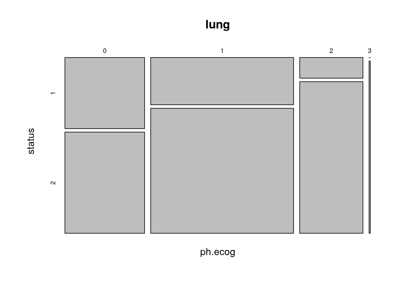
Plot control data, where a higher value is associated with better survival (status = 1).
mosaicplot(control ~ status, data = lung)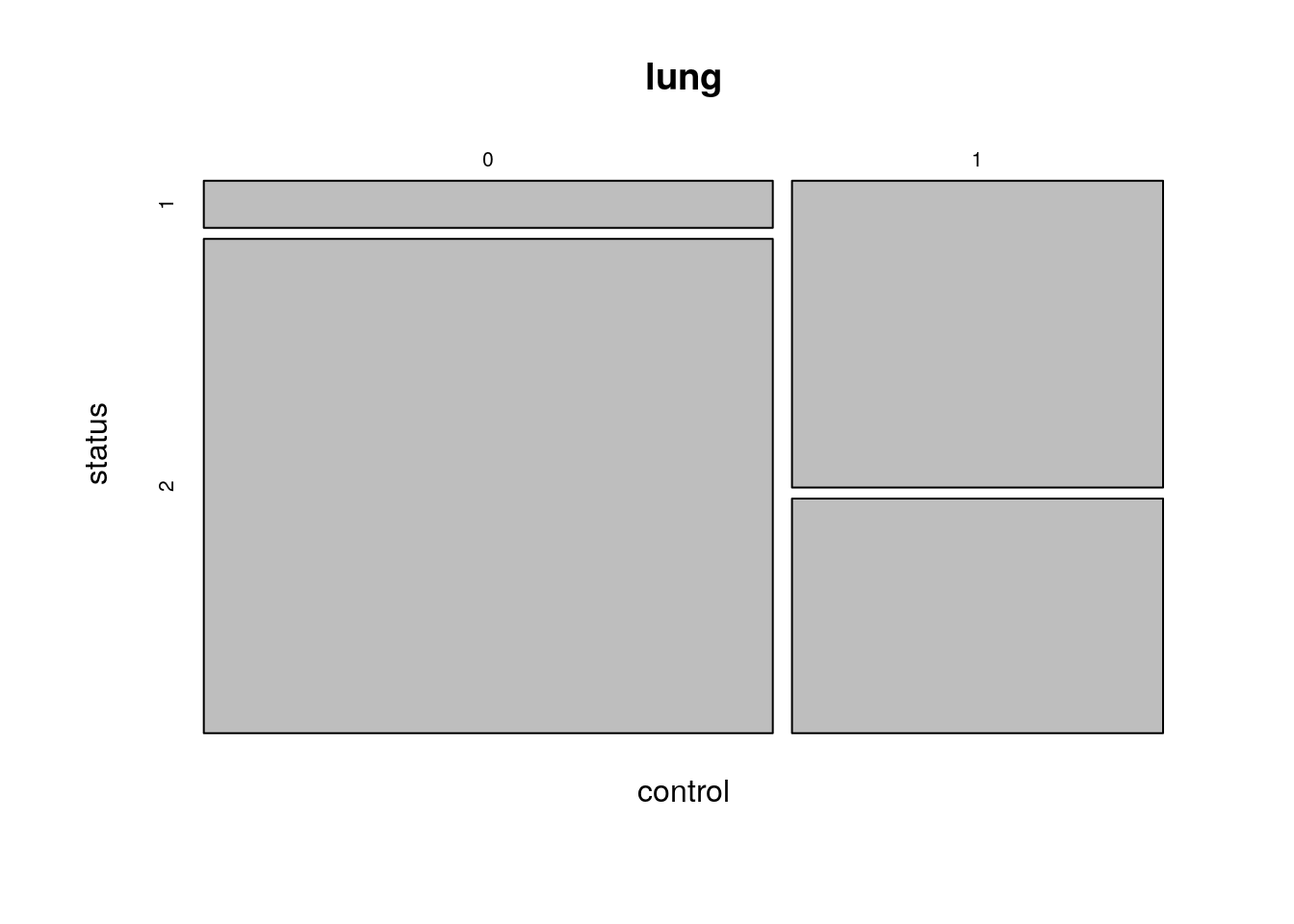
Compute survival curves
The function survfit() can be used to compute
Kaplan-Meier survival estimates. Its main arguments include:
- A survival object created using the function
Surv() - The data set containing the variables
Compute the survival probability by gender.
fit <- survfit(Surv(time, status) ~ sex, data = lung)
fit
Call: survfit(formula = Surv(time, status) ~ sex, data = lung)
n events median 0.95LCL 0.95UCL
sex=1 138 112 270 212 310
sex=2 90 53 426 348 550Use summary(fit) to get a complete summary of the
survival curves.
names(fit) [1] "n" "time" "n.risk" "n.event" "n.censor" "surv"
[7] "std.err" "cumhaz" "std.chaz" "strata" "type" "logse"
[13] "conf.int" "conf.type" "lower" "upper" "call" The surv_summary() function can also be used to get a
summary of survival curves.
fit_sum <- surv_summary(fit, data = lung)
head(fit_sum)
time n.risk n.event n.censor surv std.err upper lower strata
1 11 138 3 0 0.9782609 0.01268978 1.0000000 0.9542301 sex=1
2 12 135 1 0 0.9710145 0.01470747 0.9994124 0.9434235 sex=1
3 13 134 2 0 0.9565217 0.01814885 0.9911586 0.9230952 sex=1
4 15 132 1 0 0.9492754 0.01967768 0.9866017 0.9133612 sex=1
5 26 131 1 0 0.9420290 0.02111708 0.9818365 0.9038355 sex=1
6 30 130 1 0 0.9347826 0.02248469 0.9768989 0.8944820 sex=1
sex
1 1
2 1
3 1
4 1
5 1
6 1| Name | Details |
|---|---|
| time | the time points at which the curve has a step |
| n.risk | the number of subjects at risk at time t |
| n.event | the number of events that occurred at time t |
| n.censor | the number of censored subjects, who exit the risk set, without an event, at time t |
| surv | estimate of survival probability |
| std.err | standard error of survival |
| lower,upper | lower and upper confidence limits for the curve, respectively |
| strata | indicates stratification of curve estimation |
If strata is not NULL, there are multiple curves in the result. The levels of strata (a factor) are the labels for the curves.
Visualise survival curves
The ggsurvplot() function can be used to produce the
survival curves for the two groups of subjects.
It is possible to show:
- The 95% confidence limits of the survivor function using the
argument
conf.int = TRUE - The number and/or the percentage of individuals at risk by time
using the option
risk.table. Allowed values forrisk.tableinclude:TRUEorFALSEspecifying whether to show or not the risk table. Default isFALSEabsoluteorpercentageto show the absolute number and the percentage of subjects at risk by time, respectively. Useabs_pctto show both absolute number and percentage.
- The p-value of the Log-Rank test comparing the groups using
pval = TRUE - Horizontal/vertical line at median survival using the argument
surv.median.line. Allowed values include:none,hv,h, andv
We will plot the survival plot with the following options:
- Add risk table
- Change risk table color by groups
- Change line type by groups
- Specify median survival
- Use the
theme_bw()ggplot2 theme - Plot the number of censored subjects at time t
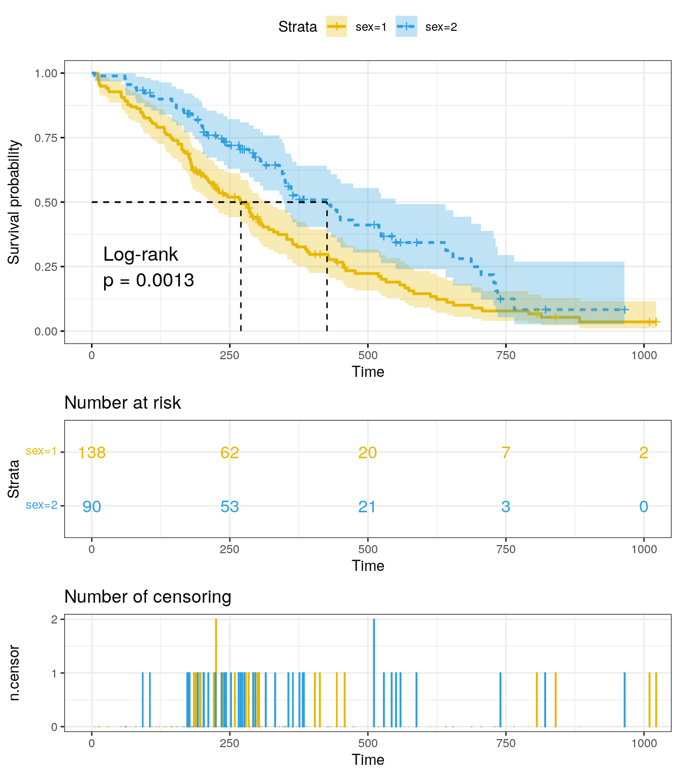
ggsurvplot(
  fit,
  pval = TRUE,
  pval.method = TRUE,
  conf.int = TRUE,
  risk.table = TRUE,
  risk.table.col = "strata",
  linetype = "strata",
  surv.median.line = "hv",
  ggtheme = theme_bw(),
  ncensor.plot = TRUE,
  palette = c("#E7B800", "#2E9FDF")
)
| Version | Author | Date |
|---|---|---|
| b1d68db | Dave Tang | 2023-11-09 |
The x-axis represents time in days, and the y-axis shows the
probability of surviving or the proportion of people surviving. The
lines represent survival curves of the two groups. A vertical drop in
the curves indicates an event, which in this case is the
status (1 = censored and 2 = dead). The vertical tick mark
on the curves means that a patient was censored at this time.
At time zero, the survival probability is 1.0. At time 250, the probability of survival is approximately 0.55 (or 55%) for sex=1 and 0.75 (or 75%) for sex=2. The median survival is approximately 270 days for sex=1 and 426 days for sex=2, suggesting a good survival for sex=2 compared to sex=1.
summary(fit)$table records n.max n.start events rmean se(rmean) median 0.95LCL 0.95UCL
sex=1 138 138 138 112 326.0841 22.91156 270 212 310
sex=2 90 90 90 53 460.6473 34.68985 426 348 550There appears to be a survival advantage for female with lung cancer compare to male. However, to evaluate whether this difference is statistically significant requires a formal statistical test.
Three often used transformations for ggsurvplot can be
specified using the argument fun:
log: log transformation of the survivor functionevent: plots cumulative events \(f(y) = 1-y\). It is also known as the cumulative incidencecumhazplots the cumulative hazard function \(f(y) = -log(y)\)
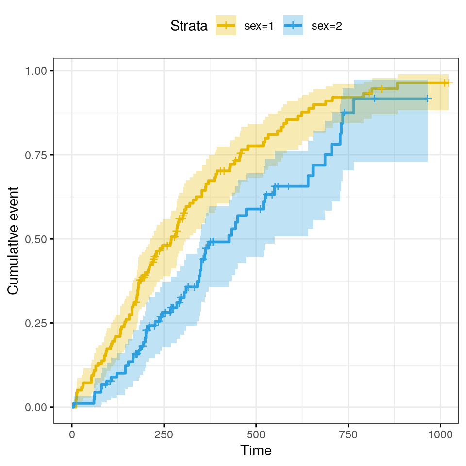
Plot cumulative events.
ggsurvplot(
  fit,
  conf.int = TRUE,
  risk.table.col = "strata",
  ggtheme = theme_bw(),
  palette = c("#E7B800", "#2E9FDF"),
  fun = "event"
)
| Version | Author | Date |
|---|---|---|
| b1d68db | Dave Tang | 2023-11-09 |
The cumulative hazard is commonly used to estimate the hazard probability. It is defined as \(H(t) = −log(S(t))\). The cumulative hazard \(H(t)\) can be interpreted as the cumulative force of mortality. In other words, it corresponds to the number of events that would be expected for each individual by time \(t\) if the event were a repeatable process.
ggsurvplot(
  fit,
  conf.int = TRUE,
  risk.table.col = "strata",
  ggtheme = theme_bw(),
  palette = c("#E7B800", "#2E9FDF"),
  fun = "cumhaz"
)
| Version | Author | Date |
|---|---|---|
| b1d68db | Dave Tang | 2023-11-09 |
Log-Rank test comparing survival curves
The log-rank test is the most widely used method of comparing two or more survival curves. The null hypothesis is that there is no difference in survival between the two groups. The log rank test is a non-parametric test, which makes no assumptions about the survival distributions.
Essentially, the log rank test compares the observed number of events in each group to what would be expected if the null hypothesis were true (i.e., if the survival curves were identical). The log rank statistic is approximately distributed as a chi-square test statistic.
The survdiff() function can be used to compute log-rank
test comparing two or more survival curves.
sex_survdiff <- survdiff(Surv(time, status) ~ sex, data = lung)
sex_survdiff
Call:
survdiff(formula = Surv(time, status) ~ sex, data = lung)
N Observed Expected (O-E)^2/E (O-E)^2/V
sex=1 138 112 91.6 4.55 10.3
sex=2 90 53 73.4 5.68 10.3
Chisq= 10.3 on 1 degrees of freedom, p= 0.001 The log rank test for difference in survival gives a p-value of 0.0013112, indicating that the sex groups differ significantly in survival.
Summary
Survival analysis is a set of statistical approaches for data analysis where the outcome variable of interest is time until an event occurs.
Survival data are generally described and modeled in terms of two related functions:
- The survivor function representing the probability that an individual survives from the time of origin to some time beyond time \(t\). It is usually estimated by the Kaplan-Meier method. The logrank test may be used to test for differences between survival curves for groups, such as treatments or gender as per this post.
- The hazard function gives the instantaneous potential of having an event at a time, given survival up to that time. It is used primarily as a diagnostic tool or for specifying a mathematical model for survival analysis.
Take home message: The survivor function focuses on not having an event and the hazard function focuses on the event occurring.
References
Cox Proportional-Hazards Model
The Cox proportional-hazards model (Cox, 1972) is essentially a regression model commonly used in medical research for investigating the association between the survival time of patients and one or more predictor variables.
In the Survival analysis in R section, we looked at Kaplan-Meier curves and logrank tests, which are examples of univariate analysis. They describe the survival according to one factor under investigation, but ignore the impact of any others. Additionally, Kaplan-Meier curves and logrank tests are useful only when the predictor variable is categorical and do not work easily for quantitative predictors such as gene expression, weight, or age.
An alternative method is the Cox proportional hazards regression analysis, which works for both quantitative predictor variables and for categorical variables. Furthermore, the Cox regression model extends survival analysis methods to assess simultaneously the effect of several risk factors on survival time.
The Cox proportional-hazards model is one of the most important methods used for modelling survival analysis data.
The need for multivariate statistical modeling
In clinical investigations, there are many situations, where several known quantities (known as covariates), potentially affecting patient prognosis; for example, comparing two groups of patients where one group has a specific genotype against those without. Furthermore, if one of the groups also contains older individuals, any difference in survival may be attributable to genotype or age (confounding) or indeed both. Hence, when investigating survival in relation to any one factor, it is often desirable to adjust for the impact of others. A statistical model can provide the effect size for each factor.
Basics of the Cox proportional hazards model
The purpose of the model is to evaluate simultaneously the effect of several factors on survival. In other words, it allows us to examine how specified factors influence the rate of a particular event happening (e.g., infection, death) at a particular point in time. This rate is commonly referred as the hazard rate. Predictor variables (or factors) are usually termed covariates in the survival-analysis literature.
The Cox model is expressed by the hazard function denoted by \(h(t)\). Briefly, the hazard function can be interpreted as the risk of dying at time \(t\). It can be estimated as follow:
\[ h(t) = h_0(t) \times exp(b_1x_1 + b_2x_2 + \ldots + b_px_p) \]
where:
- \(t\) represents the survival time
- \(h(t)\) is the hazard function determined by a set of \(p\) covariates \((x_1, x_2, \ldots, x_p)\)
- the coefficients \((b_1, b_2, \ldots, b_p)\) measure the impact (i.e., the effect size) of covariates
- the term \(h_0\) is called the baseline hazard. It corresponds to the value of the hazard if all the \(x_i\) are equal to zero (the quantity \(exp(0)\) equals 1). The \(t\) in \(h(t)\) reminds us that the hazard may vary over time.
The Cox model can be written as a multiple linear regression of the logarithm of the hazard on the variables \(x_i\), with the baseline hazard being an intercept term that varies with time.
The quantities \(exp(b_i)\) are called hazard ratios (HR). A value of \(b_i\) greater than zero, or equivalently a hazard ratio greater than one, indicates that as the value of the \(i^{th}\) covariate increases, the event hazard increases and thus the length of survival decreases.
A hazard ratio above 1 indicates a covariate that is positively associated with the event probability, and thus negatively associated with the length of survival.
In summary:
- HR = 1: No effect
- HR < 1: Reduction in the hazard
- HR > 1: Increase in hazard
In cancer studies:
- A covariate with hazard ratio > 1 (i.e.: \(b > 0\)) is called bad prognostic factor
- A covariate with hazard ratio < 1 (i.e.: \(b < 0\)) is called good prognostic factor
A key assumption of the Cox model is that the hazard curves for the groups of observations (or patients) should be proportional and cannot cross. In other words, if an individual has a risk of death at some initial time point that is twice as high as that of another individual, then at all later times the risk of death remains twice as high.
Computing the Cox model
The coxph function can be used to compute the Cox
proportional hazards regression model in R. The simplified format
is:
coxph(formula, data, method)formulaspecifies a linear model with a survival object as the response variable. The survival object is created using theSurv()functionSurv(time, event).datais a data frame that contains the variables.methodis used to specify how to handle ties. The default isefron. Other options arebreslowandexact. The defaultefronis generally preferred to the once-popularbreslowmethod and theexactmethod is much more computationally intensive.
We will compute a univariate Cox analysis.
sex_cox <- coxph(Surv(time, status) ~ sex, data = lung)
summary(sex_cox)
Call:
coxph(formula = Surv(time, status) ~ sex, data = lung)
n= 228, number of events= 165
coef exp(coef) se(coef) z Pr(>|z|)
sex -0.5310 0.5880 0.1672 -3.176 0.00149 **
---
Signif. codes: 0 '***' 0.001 '**' 0.01 '*' 0.05 '.' 0.1 ' ' 1
exp(coef) exp(-coef) lower .95 upper .95
sex 0.588 1.701 0.4237 0.816
Concordance= 0.579 (se = 0.021 )
Likelihood ratio test= 10.63 on 1 df, p=0.001
Wald test = 10.09 on 1 df, p=0.001
Score (logrank) test = 10.33 on 1 df, p=0.001The Cox regression results can be interpreted as follow:
Statistical significance. The column marked
zgives the Wald statistic value. It corresponds to the ratio of each regression coefficient to its standard error (z = coef/se(coef)). The Wald statistic evaluates, whether the beta (\(\beta\)) coefficient of a given variable is statistically significantly different from 0. From the output above, we can conclude that the variable sex have highly statistically significant coefficients.The regression coefficients. The second feature to note in the Cox model results is the the sign of the regression coefficients (
coef). A positive sign means that the hazard (risk of death) is higher, and thus the prognosis worse, for subjects with higher values of that variable. The variable sex is encoded as a numeric vector; 1: male, 2: female. The R summary for the Cox model gives the hazard ratio (HR) for the second group relative to the first group, that is, female versus male. The beta coefficient for sex = -0.53 indicates that females have lower risk of death (lower survival rates) than males, in thelungdataset.Hazard ratios. The exponentiated coefficients (exp(coef) = exp(-0.53) = 0.59), also known as hazard ratios, give the effect size of covariates. For example, being female (sex=2) reduces the hazard by a factor of 0.59, or 41%. Being female is associated with good prognostic.
Confidence intervals of the hazard ratios. The summary output also gives upper and lower 95% confidence intervals for the hazard ratio (exp(coef)), lower 95% bound = 0.4237, upper 95% bound = 0.816.
Global statistical significance of the model. Finally, the output gives p-values for three alternative tests for overall significance of the model: The likelihood-ratio test, Wald test, and score logrank statistics. These three methods are asymptotically equivalent. For large enough N, they will give similar results. For small N, they may differ somewhat. The Likelihood ratio test has better behavior for small sample sizes, so it is generally preferred.
In lung male=1 and female=2. Since the sign of the
coefficients is meaningful, it is important to figure out how the groups
are compared. As noted above, the hazard ratio is for the second group
relative to the first group. But lung$sex is a numeric and
not a factor, so it is unclear, which group is the first and which is
the second.
The coxph function works with factors and we can
explicitly state the first and second groups using the
levels option. The results are now switched around!
lung2 <- lung
lung2$sex <- factor(lung2$sex, levels = c(2, 1))
levels(lung2$sex)
[1] "2" "1"sex_cox2 <- coxph(Surv(time, status) ~ sex, data = lung2)
summary(sex_cox2)Call:
coxph(formula = Surv(time, status) ~ sex, data = lung2)
n= 228, number of events= 165
coef exp(coef) se(coef) z Pr(>|z|)
sex1 0.5310 1.7007 0.1672 3.176 0.00149 **
---
Signif. codes: 0 '***' 0.001 '**' 0.01 '*' 0.05 '.' 0.1 ' ' 1
exp(coef) exp(-coef) lower .95 upper .95
sex1 1.701 0.588 1.226 2.36
Concordance= 0.579 (se = 0.021 )
Likelihood ratio test= 10.63 on 1 df, p=0.001
Wald test = 10.09 on 1 df, p=0.001
Score (logrank) test = 10.33 on 1 df, p=0.001In addition the status is coded as 1=censored and 2=dead. If we convert the status into a factor we will get the following error:
an id statement is required for multi-state modelsIf I switch the status around, the results are reversed.
lung3 <- lung
lung3$status <- ifelse(lung3$status == 2, 1, 2)
sex_cox3 <- coxph(Surv(time, status) ~ sex, data = lung3)
summary(sex_cox3)
Call:
coxph(formula = Surv(time, status) ~ sex, data = lung3)
n= 228, number of events= 63
coef exp(coef) se(coef) z Pr(>|z|)
sex 0.6476 1.9109 0.2638 2.454 0.0141 *
---
Signif. codes: 0 '***' 0.001 '**' 0.01 '*' 0.05 '.' 0.1 ' ' 1
exp(coef) exp(-coef) lower .95 upper .95
sex 1.911 0.5233 1.139 3.205
Concordance= 0.563 (se = 0.036 )
Likelihood ratio test= 6.21 on 1 df, p=0.01
Wald test = 6.02 on 1 df, p=0.01
Score (logrank) test = 6.23 on 1 df, p=0.01Perform the univariate Cox analysis on the control data, where a higher value is associated with better survival.
control_cox <- coxph(Surv(time, status) ~ control, data = lung)
summary(control_cox)
Call:
coxph(formula = Surv(time, status) ~ control, data = lung)
n= 228, number of events= 165
coef exp(coef) se(coef) z Pr(>|z|)
control -0.8118 0.4440 0.1841 -4.411 1.03e-05 ***
---
Signif. codes: 0 '***' 0.001 '**' 0.01 '*' 0.05 '.' 0.1 ' ' 1
exp(coef) exp(-coef) lower .95 upper .95
control 0.444 2.252 0.3096 0.6369
Concordance= 0.606 (se = 0.02 )
Likelihood ratio test= 21.98 on 1 df, p=3e-06
Wald test = 19.45 on 1 df, p=1e-05
Score (logrank) test = 20.52 on 1 df, p=6e-06Perform the univariate Cox analysis on other covariates.
covariates <- c("age", "sex",  "ph.karno", "pat.karno", "ph.ecog", "wt.loss", "control")
univ_formulas <- sapply(
  covariates,
  function(x) as.formula(paste('Surv(time, status)~', x))
)

univ_models <- lapply(univ_formulas, function(x){
  coxph(x, data = lung)}
)

univ_results <- lapply(
  univ_models,
  function(x){
    x <- summary(x)
    p.value<-signif(x$wald["pvalue"], digits=2)
    wald.test<-signif(x$wald["test"], digits=2)
    beta<-signif(x$coef[1], digits=2)
    HR <-signif(x$coef[2], digits=2)
    HR.confint.lower <- signif(x$conf.int[,"lower .95"], 2)
    HR.confint.upper <- signif(x$conf.int[,"upper .95"],2)
    HR <- paste0(
      HR, " (",
      HR.confint.lower, "-", HR.confint.upper, ")"
    )
    res<-c(beta, HR, wald.test, p.value)
    names(res)<-c("beta", "HR (95% CI for HR)", "wald.test", "p.value")
    return(res)
  }
)
res <- t(as.data.frame(univ_results, check.names = FALSE))
as.data.frame(res)
beta HR (95% CI for HR) wald.test p.value
age 0.019 1 (1-1) 4.1 0.042
sex -0.53 0.59 (0.42-0.82) 10 0.0015
ph.karno -0.016 0.98 (0.97-1) 7.9 0.005
pat.karno -0.02 0.98 (0.97-0.99) 13 0.00028
ph.ecog 0.48 1.6 (1.3-2) 18 2.7e-05
wt.loss 0.0013 1 (0.99-1) 0.05 0.83
control -0.81 0.44 (0.31-0.64) 19 1e-05The variables age, sex,
ph.karno, pat.karno, and ph.ecog
have statistically significant coefficients. age and
ph.ecog have positive beta coefficients, while sex has a
negative coefficient. Thus, older age and higher ph.ecog
are associated with poorer survival, whereas being female (sex=2) is
associated with better survival.
To perform a multivariate Cox regression analysis, include the additional covariates in the formula.
res_cox <- coxph(Surv(time, status) ~ age + sex + ph.karno + pat.karno + ph.ecog + wt.loss, data =  lung)
summary(res_cox)
Call:
coxph(formula = Surv(time, status) ~ age + sex + ph.karno + pat.karno +
ph.ecog + wt.loss, data = lung)
n= 210, number of events= 148
(18 observations deleted due to missingness)
coef exp(coef) se(coef) z Pr(>|z|)
age 0.013058 1.013144 0.009866 1.324 0.185639
sex -0.625167 0.535172 0.178703 -3.498 0.000468 ***
ph.karno 0.020116 1.020320 0.010178 1.976 0.048111 *
pat.karno -0.014743 0.985365 0.007300 -2.019 0.043440 *
ph.ecog 0.675227 1.964479 0.198735 3.398 0.000680 ***
wt.loss -0.013243 0.986844 0.007009 -1.889 0.058836 .
---
Signif. codes: 0 '***' 0.001 '**' 0.01 '*' 0.05 '.' 0.1 ' ' 1
exp(coef) exp(-coef) lower .95 upper .95
age 1.0131 0.9870 0.9937 1.0329
sex 0.5352 1.8686 0.3770 0.7596
ph.karno 1.0203 0.9801 1.0002 1.0409
pat.karno 0.9854 1.0149 0.9714 0.9996
ph.ecog 1.9645 0.5090 1.3307 2.9001
wt.loss 0.9868 1.0133 0.9734 1.0005
Concordance= 0.656 (se = 0.025 )
Likelihood ratio test= 37.2 on 6 df, p=2e-06
Wald test = 36.49 on 6 df, p=2e-06
Score (logrank) test = 37.59 on 6 df, p=1e-06The p-value for all three overall tests (likelihood, Wald, and score) are significant, indicating that the model is significant. These tests evaluate the omnibus null hypothesis that all of the betas are 0. In the above example, the test statistics are in close agreement, and the omnibus null hypothesis is soundly rejected.
In the multivariate Cox analysis, the covariates sex,
ph.karno, pat.karno, and ph.ecog
remain significant (p < 0.05) and the covariate age is
no longer significant.
The p-value for sex is 0.000986, with a hazard ratio HR
= exp(coef) = 0.58, indicating a strong relationship between the
patients’ sex and decreased risk of death. The hazard ratios of
covariates are interpretable as multiplicative effects on the hazard.
For example, holding the other covariates constant, being female (sex=2)
reduces the hazard by a factor of 0.58, or 42%. We conclude that, being
female is associated with good prognostic.
Similarly, the p-value for ph.ecog is 4.45e-05, with a
hazard ratio HR = 1.59, indicating a strong relationship between the
ph.ecog value and increased risk of death. Holding the
other covariates constant, a higher value of ph.ecog is
associated with a poor survival.
By contrast, the p-value for age is now p=0.23, compared
to the univariate Cox analysis. The hazard ratio HR = exp(coef) = 1.01,
with a 95% confidence interval of 0.99 to 1.03. Because the confidence
interval for HR includes 1, these results indicate that age makes a
smaller contribution to the difference in the HR after adjusting for the
ph.ecog values and patient’s sex, and only
trend toward significance. For example, holding the other covariates
constant, an additional year of age induce daily hazard of death by a
factor of exp(beta) = 1.01, or 1%, which is not a significant
contribution.
We can visualise the predicted survival proportion at any given point
in time for a particular risk group. The survfit() function
estimates the survival proportion, by default at the mean values of
covariates.
ggsurvplot(
  survfit(res_cox),
  ggtheme = theme_minimal(),
  color = "#2E9FDF",
  data = lung
)
Warning: Now, to change color palette, use the argument palette= '#2E9FDF'
instead of color = '#2E9FDF'
Consider that, we want to assess the impact of the sex on the estimated survival probability. In this case, we construct a new data frame with two rows, one for each value of sex; the other covariates are fixed to their average values (if they are continuous variables) or to their lowest level (if they are discrete variables). For a dummy covariate, the average value is the proportion coded 1 in the data set. This data frame is passed to survfit() via the newdata argument.
sex_df <- with(
  lung,
  data.frame(
    sex = c(1, 2),
    age = rep(mean(age, na.rm = TRUE), 2),
    ph.ecog = c(1, 1),
    ph.karno = rep(mean(ph.karno, na.rm=TRUE), 2),
    pat.karno = rep(mean(pat.karno, na.rm=TRUE), 2),
    wt.loss = rep(mean(wt.loss, na.rm=TRUE), 2)
  )
)
sex_df
sex age ph.ecog ph.karno pat.karno wt.loss
1 1 62.44737 1 81.93833 79.95556 9.831776
2 2 62.44737 1 81.93833 79.95556 9.831776fit <- survfit(res_cox, newdata = sex_df)
ggsurvplot(
fit,
conf.int = TRUE,
legend.labs=c("Sex=1", "Sex=2"),
ggtheme = theme_minimal(),
data = lung
)Warning: `gather_()` was deprecated in tidyr 1.2.0.
ℹ Please use `gather()` instead.
ℹ The deprecated feature was likely used in the survminer package.
Please report the issue at <https://github.com/kassambara/survminer/issues>.
This warning is displayed once every 8 hours.
Call `lifecycle::last_lifecycle_warnings()` to see where this warning was
generated.
References
sessionInfo()R version 4.3.2 (2023-10-31)
Platform: x86_64-pc-linux-gnu (64-bit)
Running under: Ubuntu 22.04.3 LTS
Matrix products: default
BLAS: /usr/lib/x86_64-linux-gnu/openblas-pthread/libblas.so.3
LAPACK: /usr/lib/x86_64-linux-gnu/openblas-pthread/libopenblasp-r0.3.20.so; LAPACK version 3.10.0
locale:
[1] LC_CTYPE=en_US.UTF-8 LC_NUMERIC=C
[3] LC_TIME=en_US.UTF-8 LC_COLLATE=en_US.UTF-8
[5] LC_MONETARY=en_US.UTF-8 LC_MESSAGES=en_US.UTF-8
[7] LC_PAPER=en_US.UTF-8 LC_NAME=C
[9] LC_ADDRESS=C LC_TELEPHONE=C
[11] LC_MEASUREMENT=en_US.UTF-8 LC_IDENTIFICATION=C
time zone: Etc/UTC
tzcode source: system (glibc)
attached base packages:
[1] stats graphics grDevices utils datasets methods base
other attached packages:
[1] survminer_0.4.9 ggpubr_0.6.0 ggplot2_3.4.4 survival_3.5-7
[5] workflowr_1.7.1
loaded via a namespace (and not attached):
[1] gtable_0.3.4 xfun_0.41 bslib_0.6.1 processx_3.8.3
[5] rstatix_0.7.2 lattice_0.21-9 callr_3.7.3 vctrs_0.6.5
[9] tools_4.3.2 ps_1.7.5 generics_0.1.3 tibble_3.2.1
[13] fansi_1.0.6 highr_0.10 pkgconfig_2.0.3 Matrix_1.6-1.1
[17] data.table_1.14.10 lifecycle_1.0.4 farver_2.1.1 compiler_4.3.2
[21] stringr_1.5.1 git2r_0.33.0 munsell_0.5.0 getPass_0.2-4
[25] carData_3.0-5 httpuv_1.6.13 htmltools_0.5.7 sass_0.4.8
[29] yaml_2.3.8 crayon_1.5.2 later_1.3.2 pillar_1.9.0
[33] car_3.1-2 jquerylib_0.1.4 whisker_0.4.1 tidyr_1.3.0
[37] cachem_1.0.8 abind_1.4-5 km.ci_0.5-6 commonmark_1.9.0
[41] tidyselect_1.2.0 digest_0.6.33 stringi_1.8.3 dplyr_1.1.4
[45] purrr_1.0.2 labeling_0.4.3 splines_4.3.2 rprojroot_2.0.4
[49] fastmap_1.1.1 grid_4.3.2 colorspace_2.1-0 cli_3.6.2
[53] magrittr_2.0.3 utf8_1.2.4 broom_1.0.5 withr_2.5.2
[57] scales_1.3.0 promises_1.2.1 backports_1.4.1 rmarkdown_2.25
[61] httr_1.4.7 ggtext_0.1.2 gridExtra_2.3 ggsignif_0.6.4
[65] zoo_1.8-12 evaluate_0.23 knitr_1.45 KMsurv_0.1-5
[69] markdown_1.12 survMisc_0.5.6 rlang_1.1.2 gridtext_0.1.5
[73] Rcpp_1.0.11 xtable_1.8-4 glue_1.6.2 xml2_1.3.6
[77] rstudioapi_0.15.0 jsonlite_1.8.8 R6_2.5.1 fs_1.6.3