Tissue specificity
2023-10-13
Last updated: 2023-10-13
Checks: 7 0
Knit directory: muse/
This reproducible R Markdown analysis was created with workflowr (version 1.7.1). The Checks tab describes the reproducibility checks that were applied when the results were created. The Past versions tab lists the development history.
Great! Since the R Markdown file has been committed to the Git repository, you know the exact version of the code that produced these results.
Great job! The global environment was empty. Objects defined in the global environment can affect the analysis in your R Markdown file in unknown ways. For reproduciblity it’s best to always run the code in an empty environment.
The command set.seed(20200712) was run prior to running
the code in the R Markdown file. Setting a seed ensures that any results
that rely on randomness, e.g. subsampling or permutations, are
reproducible.
Great job! Recording the operating system, R version, and package versions is critical for reproducibility.
Nice! There were no cached chunks for this analysis, so you can be confident that you successfully produced the results during this run.
Great job! Using relative paths to the files within your workflowr project makes it easier to run your code on other machines.
Great! You are using Git for version control. Tracking code development and connecting the code version to the results is critical for reproducibility.
The results in this page were generated with repository version cb62ae5. See the Past versions tab to see a history of the changes made to the R Markdown and HTML files.
Note that you need to be careful to ensure that all relevant files for
the analysis have been committed to Git prior to generating the results
(you can use wflow_publish or
wflow_git_commit). workflowr only checks the R Markdown
file, but you know if there are other scripts or data files that it
depends on. Below is the status of the Git repository when the results
were generated:
Ignored files:
    Ignored:    .Rhistory
    Ignored:    .Rproj.user/
    Ignored:    r_packages_4.3.0/
    Ignored:    r_packages_4.3.1/

Untracked files:
    Untracked:  analysis/cell_ranger.Rmd
    Untracked:  analysis/complex_heatmap.Rmd
    Untracked:  analysis/sleuth.Rmd
    Untracked:  analysis/tss_xgboost.Rmd
    Untracked:  code/multiz100way/
    Untracked:  data/HG00702_SH089_CHSTrio.chr1.vcf.gz
    Untracked:  data/HG00702_SH089_CHSTrio.chr1.vcf.gz.tbi
    Untracked:  data/ncrna_NONCODE[v3.0].fasta.tar.gz
    Untracked:  data/ncrna_noncode_v3.fa
    Untracked:  data/netmhciipan.out.gz
    Untracked:  data/test
    Untracked:  export/davetang039sblog.WordPress.2023-06-30.xml
    Untracked:  export/output/
    Untracked:  women.json

Unstaged changes:
    Modified:   analysis/graph.Rmd
Note that any generated files, e.g. HTML, png, CSS, etc., are not included in this status report because it is ok for generated content to have uncommitted changes.
These are the previous versions of the repository in which changes were
made to the R Markdown (analysis/tissue.Rmd) and HTML
(docs/tissue.html) files. If you’ve configured a remote Git
repository (see ?wflow_git_remote), click on the hyperlinks
in the table below to view the files as they were in that past version.
| File | Version | Author | Date | Message |
|---|---|---|---|---|
| Rmd | cb62ae5 | Dave Tang | 2023-10-13 | Compare different metrics |
| html | 8dfc41d | Dave Tang | 2023-10-11 | Build site. |
| Rmd | 803f3ba | Dave Tang | 2023-10-11 | Other metrics |
| html | d5f2d49 | Dave Tang | 2023-10-11 | Build site. |
| Rmd | 7c1bdcd | Dave Tang | 2023-10-11 | Tissue specificity |
A key measure in information theory is entropy, which is:
“The amount of uncertainty involved in a random process; the lower the uncertainty, the lower the entropy.”
For example, there is lower entropy in a fair coin flip versus a fair die roll since there are more possible outcomes with a die roll \({1, 2, 3, 4, 5, 6}\) compared to a coin flip \({H, T}\).
Entropy is measured in bits, which has a single binary value of either 1 or 0. Since a coin toss has only two outcomes, each toss has one bit of information. However, if the coin is not fair, meaning that it is biased towards either heads or tails, there is less uncertainty, i.e. lower entropy; if a die lands on heads 60% of the time, we are more certain of heads than in a fair die (50% heads).
There is a nice example on the Information Content Wikipedia page explaining the relationship between entropy (uncertainty) and information content.
For example, quoting a character (the Hippy Dippy Weatherman) of comedian George Carlin, “Weather forecast for tonight: dark. Continued dark overnight, with widely scattered light by morning.” Assuming one not residing near the Earth’s poles or polar circles, the amount of information conveyed in that forecast is zero because it is known, in advance of receiving the forecast, that darkness always comes with the night.
There is no uncertainty in the above statement hence that piece of information has 0 bits.
Mathematically, the Shannon entropy is defined as:
\[ -\sum_{i=1}^n p(x_i) log_{b}p(x_i) \]
Let’s test this out in R using the coin flip example above.
Firstly let’s define the entropy function according to
the formula above.
entropy <- function(x){
  -sum(log2(x)*x)
}
Generate 100 fair coin tosses.
set.seed(1984)
fair_res <- rbinom(n = 100, size = 1, prob = 0.5)
prop.table(table(fair_res))
fair_res
0 1
0.48 0.52 Calculate Shannon entropy of fair coin tosses.
entropy(as.vector(prop.table(table(fair_res))))[1] 0.9988455Generate 100 biased coin tosses.
set.seed(1984)
unfair_res <- rbinom(n = 100, size = 1, prob = 0.2)
prop.table(table(unfair_res))
unfair_res
0 1
0.76 0.24 Calculate Shannon entropy of biased coin tosses.
entropy(as.vector(prop.table(table(unfair_res))))[1] 0.7950403A biased coin will is more predicable, i.e. has less uncertainty, and therefore has less entropy than a fair coin.
In fact a fair coin has the highest entropy. This makes sense because when it’s 50/50, it is the most uncertain!
x <- seq(0.05, 0.95, 0.05)
y <- 1 - x
e <- sapply(seq_along(x), function(i) entropy(c(x[i], y[i])))

plot(x, e, xlab = "Probability of heads", ylab = "Entropy", pch = 16, xaxt = 'n')
axis(side=1, at=x)
abline(v = 0.5, lty = 3)
abline(h = 1, lty = 3)
| Version | Author | Date |
|---|---|---|
| d5f2d49 | Dave Tang | 2023-10-11 |
Tissue specificity
What does all this have to do with measuring tissue specificity? I came across this paper: Promoter features related to tissue specificity as measured by Shannon entropy and it spurred me to learn about entropy. Basically, if a gene is expressed in a tissue specific manner, we are more certain of its expression and hence there is lower entropy.
Let’s begin by defining a Shannon entropy function for use with
tissue expression. The code is from the R
help mail. This function includes a simple normalisation method of
normalising each value by the sum. In addition, if any value is less
than 0 or if the sum of all values is less than or equal to zero, the
function will return an NA.
shannon.entropy <- function(p){
   if (min(p) < 0 || sum(p) <= 0) return(NA)
   p.norm <- p[p>0]/sum(p)
   -sum(log2(p.norm)*p.norm)
}
Let’s imagine we have 30 samples and we have a gene that is ubiquitously expressed.
set.seed(1984)
all_gene <- rnorm(n = 30, mean = 50, sd = 15)
shannon.entropy(all_gene)
[1] 4.854579A ubiquitously expressed gene that is highly expressed in one sample.
all_gene_one_higher <- all_gene
all_gene_one_higher[30] <- 100
shannon.entropy(all_gene_one_higher)
[1] 4.842564Higher expression in half of the samples.
set.seed(1984)
half_gene <- c(
  rnorm(n = 15, mean = 50, sd = 10),
  rnorm(n = 15, mean = 5, sd = 1)
)
shannon.entropy(half_gene)
[1] 4.319041Expression only in one sample.
one_gene <- rep(0, 29)
one_gene[30] <- 50
shannon.entropy(one_gene)
[1] 0Expression much higher in one sample.
one_gene_with_bg <- rep(1, 29)
one_gene_with_bg[30] <- 50
shannon.entropy(one_gene_with_bg)
[1] 2.73172Expression only in three samples.
three_gene <- c(rep(1,27), 25, 65, 100)
shannon.entropy(three_gene)
[1] 2.360925Equal expression in all samples; note that the Shannon entropy will be the same regardless of the expression strength.
all_gene_equal <- rep(50, 30)
shannon.entropy(all_gene_equal)
[1] 4.906891Plot the expression patterns for the 6 scenarios.
plot_entropy <- function(x){
  barplot(x, main = round(shannon.entropy(x), 3), xlab = 'Samples', ylab = 'Expression')
}

par(mfrow=c(2,3))
examples <- list(all_gene_equal, all_gene, all_gene_one_higher, half_gene, three_gene, one_gene)
invisible(sapply(examples, plot_entropy))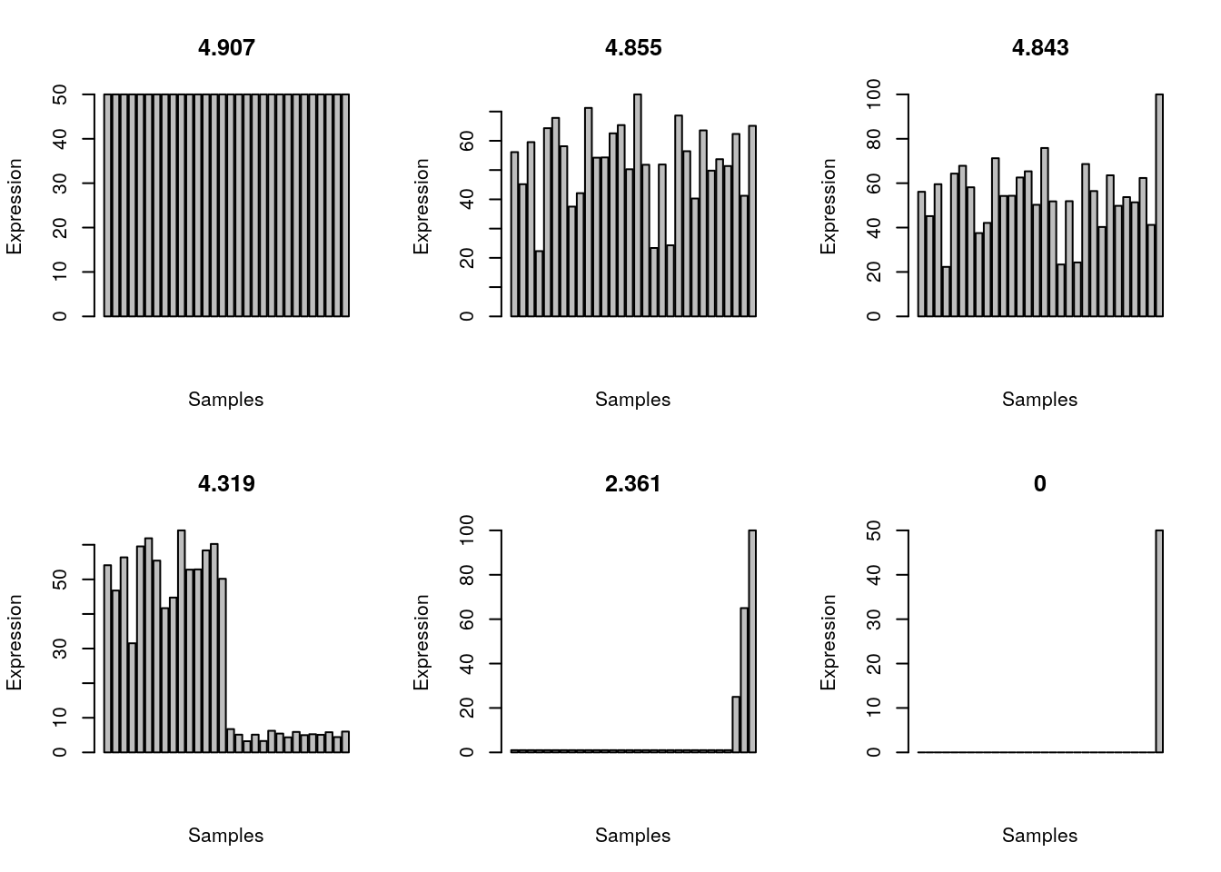
| Version | Author | Date |
|---|---|---|
| d5f2d49 | Dave Tang | 2023-10-11 |
Other tissue specificity metrics
Metrics and code from A benchmark of gene expression tissue-specificity metrics.
Tau:
\[ \tau = \frac{\sum_{i=1}^n (1 - \widehat x_i)}{n-1}; \widehat x_i = \frac{x_i}{\max_{1\le i \le n} (x_i)}\]
Implementation in R.
tau <- function(x){
  x <- (1-(x/max(x)))
  res <- sum(x, na.rm=TRUE)
  res/(length(x)-1)
}

sapply(examples, tau)
[1] 0.0000000 0.3114333 0.4739504 0.5681687 0.9596552 1.0000000EE score (summary of the expression of all genes in tissue \(i\)):
\[ EE = \frac{x_i}{\sum^n_{i=1}x_i \times \frac{s_i}{\sum^n_{i=1} s_i}} = \frac{\sum^n_{i=1} s_i}{s_i} \times \frac{x_i}{\sum^n_{i=1}x_i}s_i \]
No implementation yet as this metric requires expression data.
TSI:
\[ TSI = \frac{\max_{1 \le i \le n}(x_i)}{\sum^n_{i=1}x_i} \]
Implementation in R.
tsi <- function(x){
  max(x) / sum(x)
}

sapply(examples, tsi)
[1] 0.03333333 0.04769073 0.06151788 0.07394751 0.46082949 1.00000000Gini coefficient, where \(x_i\) has to be ordered from least to greatest:
\[ Gini = \frac{n + 1}{n} - \frac{2 \sum^n_{i=1} (n + 1 - i) x_i}{n \sum^n_{i=1}x_i} \]
Implementation in R (the gini function is missing in the
supplementary data of the paper and the loaded packages do not have this
function, so it is unclear where gini is from.). There is a
gini function in the reldist
package, which computes the Gini coefficient.
reldist::ginifunction (x, weights = rep(1, length = length(x)))
{
ox <- order(x)
x <- x[ox]
weights <- weights[ox]/sum(weights)
p <- cumsum(weights)
nu <- cumsum(weights * x)
n <- length(nu)
nu <- nu/nu[n]
sum(nu[-1] * p[-n]) - sum(nu[-n] * p[-1])
}
<bytecode: 0x5597500b1e80>
<environment: namespace:reldist>Calculate Gini coefficients (using the reldist code) for
the examples. (To save you from installing reldist, I’ve
copied the code.)
gini <- function (x, weights = rep(1, length = length(x))) {
  # code is from the reldist package by Mark S. Handcock
  # https://cran.r-project.org/web/packages/reldist/index.html
  ox <- order(x)
  x <- x[ox]
  weights <- weights[ox]/sum(weights)
  p <- cumsum(weights)
  nu <- cumsum(weights * x)
  n <- length(nu)
  nu <- nu/nu[n]
  sum(nu[-1] * p[-n]) - sum(nu[-n] * p[-1])
}

sapply(examples, gini)
[1] 0.0000000 0.1410784 0.1578373 0.4552432 0.7986175 0.9666667Shannon entropy:
\[ H_g = - \sum^n_{i=1} p_i \times log_2(p_i); p_i = \frac{x_i}{\sum^n_{i=1}x_i} \]
Implementation in R.
hg <- function(x, norm = FALSE){
  p <- x / sum(x)
  res <- -sum(p*log2(p), na.rm=TRUE)
  if(norm){
    res <- 1 - (res/log2(length(p)))
  }
  res
}

sapply(examples, hg)
[1] 4.906891 4.854579 4.842564 4.319041 2.360925 0.000000sapply(examples, hg, norm = TRUE)[1] 0.00000000 0.01066085 0.01310950 0.11980089 0.51885522 1.00000000The z-score can be implemented in two ways: either only over-expressed genes are defined as tissue specific or the absolute distance from the mean is used, so that under-expressed genes are also defined as tissue specific.
\[ \zeta = \frac{x_i - \mu}{\sigma} \]
SPM:
\[ SPM = \frac{x_i^2}{\sum^n_{i=1}x^2_i} \]
Implementation in R.
spm <- function(x, norm=TRUE){
  res <- x^2/sum(x^2)
  if (norm){
    res <- max(res)
  }
  res
}

sapply(examples, spm)
[1] 0.03333333 0.06404100 0.10458125 0.09543494 0.67217853 1.00000000PEM estimates how different the expression of the gene is relative to an expected expression, under the assumption of uniform expression in all tissues. \(s_i\) is the summary of the expression of all genes in tissue \(i\).
\[ PEM = log_{10} \left( \frac{\sum^n_{i=1}}{s_i} \times \frac{x_i}{\sum^n_{i=1} x_i} \right) \]
No implementation yet as this metric requires expression data.
Comparing metrics
Compare the metrics.
my_metrics <- data.frame(
  eg = c('identical', 'all_exp', 'all_exp_one_higher', 'half_exp', 'three_exp', 'one_exp'),
  tau = sapply(examples, tau),
  tsi = sapply(examples, tsi),
  gini = sapply(examples, gini),
  hg = sapply(examples, hg, norm=TRUE),
  spm = sapply(examples, spm)
)

pivot_longer(my_metrics, -eg, names_to = "metrics") |>
  mutate(eg = factor(eg, levels = unique(eg))) |>
  ggplot(data = _, aes(eg, value, group = metrics, colour = metrics)) +
  geom_line() +
  geom_point() +
  theme_minimal()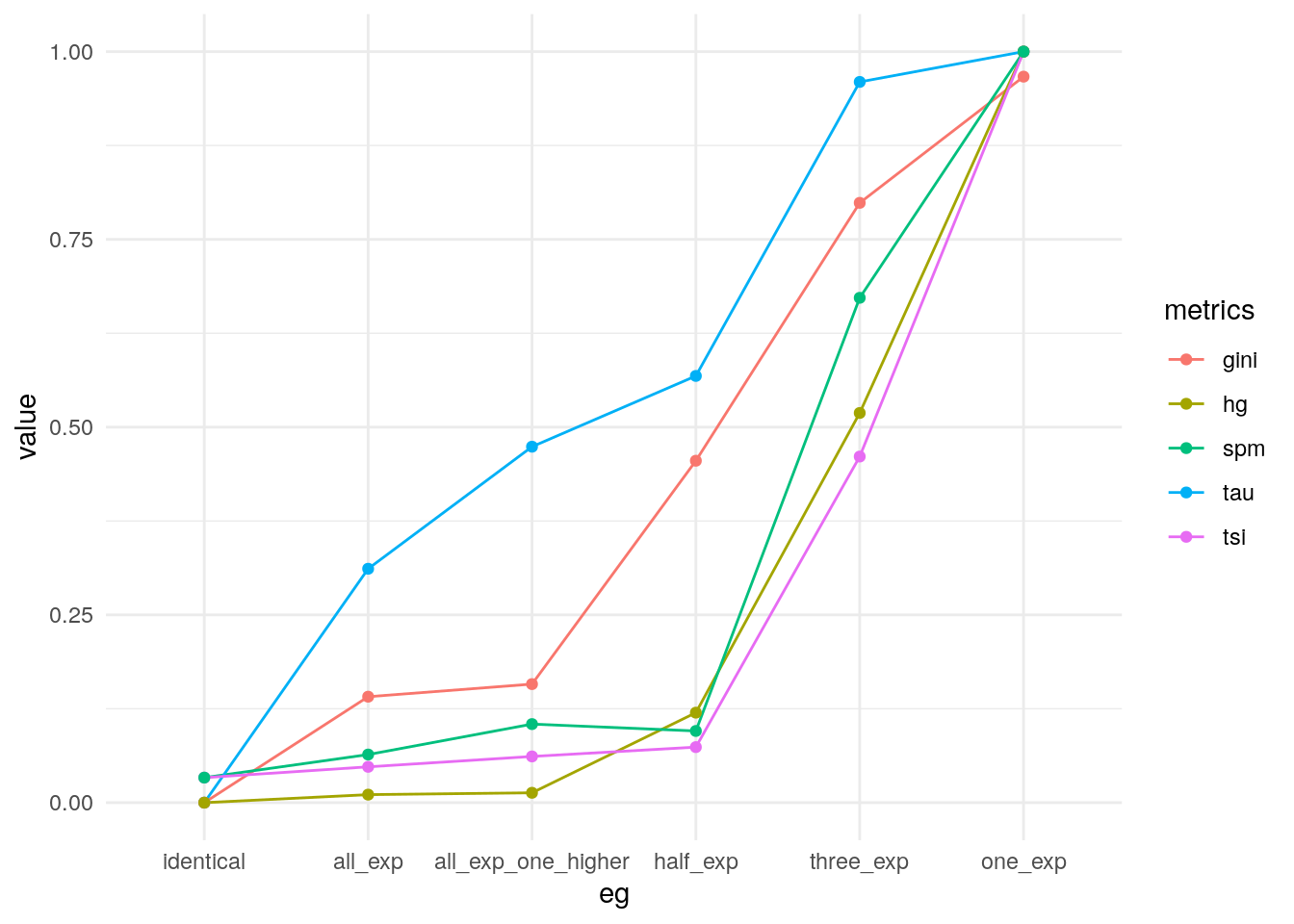
Taking the average of all metrics.
my_metrics$mean <- apply(my_metrics[, -1], 1, mean)
my_metrics$median <- apply(my_metrics[, -1], 1, median)

pivot_longer(my_metrics, -eg, names_to = "metrics") |>
  mutate(eg = factor(eg, levels = unique(eg))) |>
  ggplot(data = _, aes(eg, value, group = metrics, colour = metrics)) +
  geom_line() +
  geom_point() +
  theme_minimal()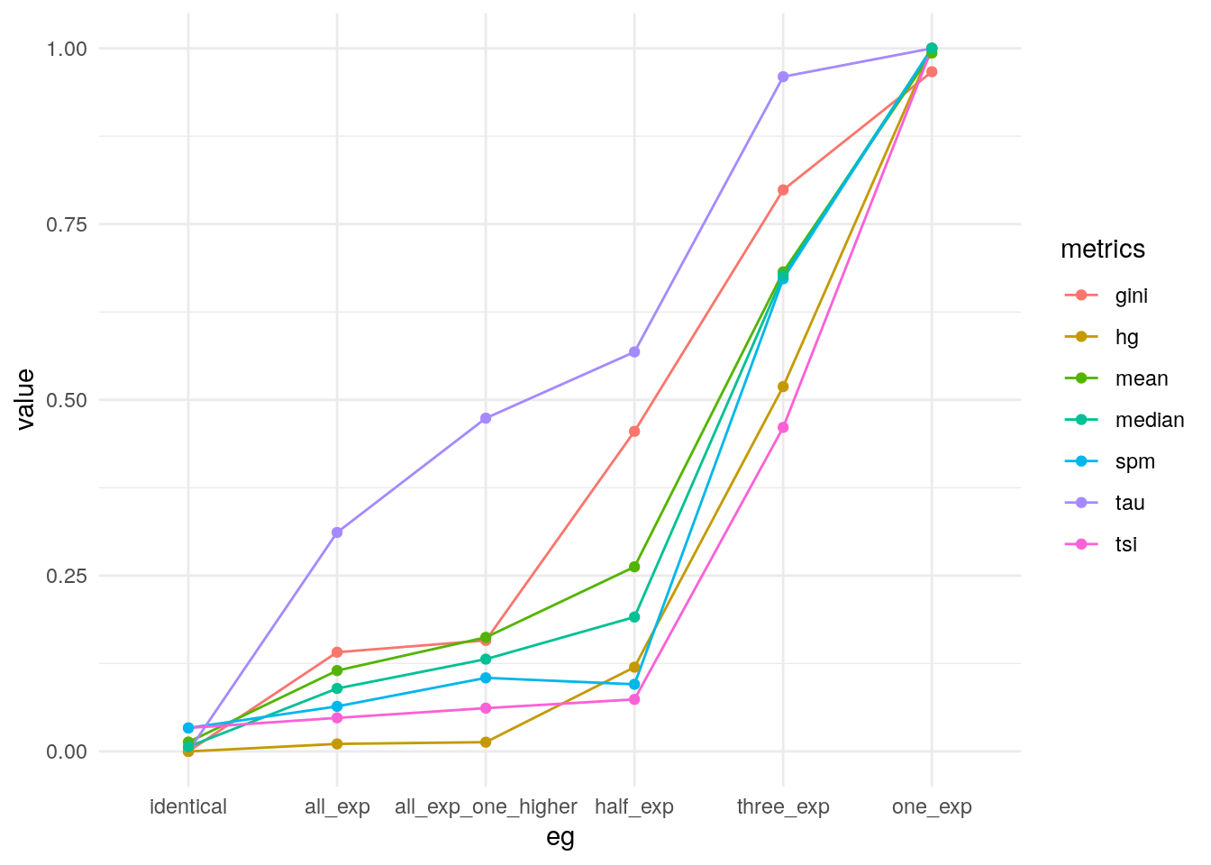
Summary
Equal expression amongst the 30 libraries resulted in a Shannon entropy of ~4.91 bits; this is similar to an even coin toss. This is close to 5 bits because we need 5 bits to transfer information on 30 samples. The more specific a gene is expressed, the less uncertainty, and therefore the lower the entropy.
sessionInfo()R version 4.3.1 (2023-06-16)
Platform: x86_64-pc-linux-gnu (64-bit)
Running under: Ubuntu 22.04.3 LTS
Matrix products: default
BLAS: /usr/lib/x86_64-linux-gnu/openblas-pthread/libblas.so.3
LAPACK: /usr/lib/x86_64-linux-gnu/openblas-pthread/libopenblasp-r0.3.20.so; LAPACK version 3.10.0
locale:
[1] LC_CTYPE=en_US.UTF-8 LC_NUMERIC=C
[3] LC_TIME=en_US.UTF-8 LC_COLLATE=en_US.UTF-8
[5] LC_MONETARY=en_US.UTF-8 LC_MESSAGES=en_US.UTF-8
[7] LC_PAPER=en_US.UTF-8 LC_NAME=C
[9] LC_ADDRESS=C LC_TELEPHONE=C
[11] LC_MEASUREMENT=en_US.UTF-8 LC_IDENTIFICATION=C
time zone: Etc/UTC
tzcode source: system (glibc)
attached base packages:
[1] stats graphics grDevices utils datasets methods base
other attached packages:
[1] lubridate_1.9.3 forcats_1.0.0 stringr_1.5.0 dplyr_1.1.3
[5] purrr_1.0.2 readr_2.1.4 tidyr_1.3.0 tibble_3.2.1
[9] ggplot2_3.4.3 tidyverse_2.0.0 workflowr_1.7.1
loaded via a namespace (and not attached):
[1] gtable_0.3.4 QuickJSR_1.0.6 xfun_0.40
[4] bslib_0.5.1 processx_3.8.2 inline_0.3.19
[7] lattice_0.21-8 callr_3.7.3 tzdb_0.4.0
[10] vctrs_0.6.3 tools_4.3.1 ps_1.7.5
[13] densEstBayes_1.0-2.2 generics_0.1.3 parallel_4.3.1
[16] stats4_4.3.1 fansi_1.0.5 pkgconfig_2.0.3
[19] Matrix_1.5-4.1 RcppParallel_5.1.7 lifecycle_1.0.3
[22] farver_2.1.1 compiler_4.3.1 git2r_0.32.0
[25] munsell_0.5.0 codetools_0.2-19 getPass_0.2-2
[28] httpuv_1.6.11 htmltools_0.5.6.1 sass_0.4.7
[31] yaml_2.3.7 crayon_1.5.2 later_1.3.1
[34] pillar_1.9.0 jquerylib_0.1.4 whisker_0.4.1
[37] cachem_1.0.8 StanHeaders_2.26.28 nlme_3.1-162
[40] rstan_2.26.23 tidyselect_1.2.0 digest_0.6.33
[43] stringi_1.7.12 labeling_0.4.3 splines_4.3.1
[46] rprojroot_2.0.3 fastmap_1.1.1 grid_4.3.1
[49] colorspace_2.1-0 cli_3.6.1 magrittr_2.0.3
[52] loo_2.6.0 pkgbuild_1.4.2 reldist_1.7-2
[55] utf8_1.2.3 withr_2.5.1 prettyunits_1.2.0
[58] scales_1.2.1 promises_1.2.1 timechange_0.2.0
[61] rmarkdown_2.25 httr_1.4.7 matrixStats_1.0.0
[64] gridExtra_2.3 hms_1.1.3 evaluate_0.22
[67] knitr_1.44 mgcv_1.8-42 rstantools_2.3.1.1
[70] rlang_1.1.1 Rcpp_1.0.11 glue_1.6.2
[73] rstudioapi_0.15.0 jsonlite_1.8.7 R6_2.5.1
[76] fs_1.6.3